|
October 4, 1965 Electronics
") [Table of Contents] [Table of Contents]
Wax nostalgic about and learn from the history of early electronics.
See articles from Electronics,
published 1930 - 1988. All copyrights hereby acknowledged.
|
Here is a good, brief introduction
to harmonic and intermodulation distortion measurement methods that were commonly
used in the 1960s. Total harmonic distortion (THD) was used often, especially for
audio equipment, which of course most frequency conversion circuits ultimately were
in the era since digital data transmission over the air was not too common. Author
Charles Moore worked for Hewlett-Packard (HP) and references HP
Application Note 15, "Distortion and Intermodulation" which,
thankfully, is made available by The HP Memory Project website.
In fact, a complete list of all the vintage app notes are available on
this page by downloading the PDF files. I highly
recommend that you download and save all you think you might ever want because as
with most things on the Web, they could disappear at any time. Some have been
captured on the Archive.org website (I just now had it save
AN-15 for time immemorial).
Two Ways to Measure Distortion
 Its cause, system nonlinearity, may be calculated
from the output harmonics of a single signal, or from the intermodulation of two. Its cause, system nonlinearity, may be calculated
from the output harmonics of a single signal, or from the intermodulation of two.
By Charles R. Moore
Loveland division, Hewlett-Packard Company Loveland, Colorado
The goal of audio and communications equipment is to reproduce input signals
faithfully at the output. But system nonlinearity changes the waveshape of the signals;
the resulting additional frequencies at the output are a measure of the distortion.
Poor reproduction brought about by distortion will appear to the user of audio equipment
as a change in the quality of musical instruments, or as noise; to the user of communications
gear, it may also appear as channel crosstalk
It is necessary to identify nonlinear distortion before it can be eliminated.
Two methods are in common use - total harmonic distortion analysis and intermodulation
distortion analysis. The choice depends primarily on the characteristics of the
system being tested and the information desired.
Linear System Theory
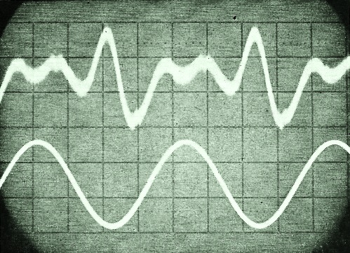
Output signal of nonlinear system, with the fundamental filtered
out, is the lower trace on the oscilloscope screen. The residual output shows that
seemingly pure sine wave does in fact contain harmonics.
Each input to a perfectly linear system produces a proportional output. For example,
if an input f1(t) produces an output g1(t), and a second input
f2(t) produces an output g2(t), the sum, f1(t)
+ f2(t), must produce g1(t) + g2(t) at the output.
The output of the system can then be defined as
G (jω) = H (jω) F (jω)
where F (jω) is the frequency spectrum of f(t), G (jω) the frequency
spectrum of g(t), and H(jω) the transfer function of the system, which has
finite gain at all frequencies. For every perfectly linear system, therefore, all
frequencies in the input will appear at the output, changed only by a scale factor;
no frequency that is not in the input can appear at the output.
For a perfectly linear amplifier, the expression is eo = Aein,
where ein is the voltage at the input, eo the voltage at the
output, and A the transfer function - in this case the gain of the amplifier. A
nonlinear amplifier, however, produces harmonics at the output, which can be characterized
by the power series expansion of its transfer function:
eo = A1ein + A2ein2
+ A3ein3 + ... + Aneinn
The purpose of any distortion measurement is to determine the value of the coefficients
of the terms in the series. As an example, if the input signal is
ein = e1 sin ω1t
+ e2 sin ω2t
then the output, eo, expanded into a Taylor power series, becomes:
DC Component

Fundamental Component

2nd and 3rd Harmonic cComponents

Intermodulation Components
If proper care has been taken during the design of a system, nonlinearity will
not be too severe. It is practical to assume that the distortion is less than 10%,
so the terms of the expansion higher than the third power have been neglected.
Analysis of the series expansion shows that the relative amplitude of the second
and third harmonic terms generated will vary directly with the input signal level.
For second harmonics, the amplitude is proportional to e12
or e22. These terms will, therefore, vary 2 decibels per decibel
of signal level change. Correspondingly, the third harmonic terms will vary 3 db
per decibel of signal. level change.
For the intermodulation terms, a frequency of the form aω1 +
bω2 varies as e1|a| e2|b|. For
example, the frequency 2ω1 - ω2 has an amplitude
proportional to e12 e2 and will vary 2 db per decibel
of signal-level change in e1, and 1 db per decibel of change in e2.
Thus, the power series defines the nonlinearity in terms of easily recognized
frequency components, whose dependence on signal level can be readily determined.
Total Harmonic Distortion Analysis
Total harmonic distortion analysis requires only one signal source. Because of
the system nonlinearity, simple harmonics of the input signal are generated at the
output. The measurement technique compares the amplitude of the harmonics to that
of the original signal at the output, where the original signal becomes the fundamental
frequency of the harmonics. The defining equation is
total harmonic distortion = 
A frequency-selective voltmeter is needed to measure the fundamental; and either
a selective voltmeter with a wide dynamic range or a frequency rejection circuit
with a true rms detector to measure the harmonics. The frequency rejection circuit
nulls the fundamental and passes its harmonics to the detector with no attenuation,
so the ratio between the fundamental and harmonics can be determined.
A less expensive way to measure the total harmonic distortion, however, is to
use a rejection filter and a broadband detector. Since the fundamental is not directly
measured, the equation becomes
THD = 
If the distortion is less than 10%, the denominator of equation 2 will be within
1/2% of the denominator in equation 1, which is as accurate as any frequency selective
voltmeter.
To cut costs further, most manufacturers use an averaging detector instead of
a broadband detector. Under certain conditions, this can lead to reading errors
in the null that are 20% to 30% low, since the averaging detector responds to the
area of the rectified waveform and not to the instantaneous power of the wave shape.
Even so, these types of errors are not considered significant; they affect only
the over-all percentage of harmonics present in the output signal and not the individual
terms, and the percentage is small. For example, a 20% error in reading the null
of a system with 0.1% harmonics results in reading of 0.08% instead.
A more important error, much larger than the metering error, is caused by the
attenuation of the harmonics by the rejection circuit. This error normally effects
the second harmonics more than the higher ones. However, manufacturers of these
circuits generally specify the second-harmonic attenuation, which makes it easy
to compensate mathematically for the error in the readings.
Disharmonies
There are two difficulties in making total harmonic distortion measurements.
First, to get a measurement within the desired accuracy, the harmonic content of
the test signal must be not more than a third of the distortion expected to be caused
by the system. Second, the chore of nulling the fundamental can be time-consuming.
Oscillators that meet the distortion requirements and automatic nulling equipment,
which has recently become available, can overcome the difficulties.
The total harmonic method is very useful when testing low-distortion circuits,
which require a large amount of negative feedback and must be unconditionally stable.
It is important that oscillations that occur in these circuits be detected. In a
TH system, the harmonics can be viewed on an oscilloscope, with the fundamental
filtered out. Not only can the character of the distortion be easily determined,
but residual oscillations that would have been much harder to find with a wave analyzer,
and are too small in comparison to the fundamental to be detected on an oscilloscope,
can be viewed.
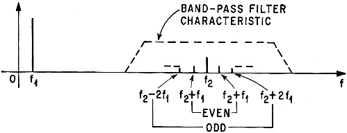
Intermodulation Distortion
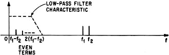
In the CCIF method of distortion measurement, two signals are
applied to the system under test. The diagram above shows how the low-pass filter
separates the low-frequency intermodulation terms from these two signals. The amplitudes
of the intermodulation, or difference terms, can be compared with that of the input
signals. The lower frequency intermodulation terms are only even.
Two signals, f1 and f2, are used in the
SMPTE method, with one having 50 times the frequency and one-quarter of the magnitude
of the other. The frequencies of interest are restricted, as shown in the diagram,
to a pass-band that is 20 times the higher frequency and centered around it. The
envelope of these terms is then used to determine the modulation index of the higher
frequency, f2 in the above diagram.
Only the SMPTE method of intermodulation distortion measurement
and the harmonic distortion technique measure both odd and even order nonlinearities.
When used to analyze amplifiers, each method defined the non-linearities of the
system in the same manner and gave the same information. They only differed by a
scale factor.
There are three major methods of making intermodulation distortion measurements.
In the Comité Consultatif International Téléphonique (CCIF)
method, two high-frequency signals with amplitudes e1 and e2
are applied to the amplifier under test. The difference between their frequencies
must lie within the amplifier's passband. The low-frequency difference products
are extracted from the output signal with a low-pass filter, and their amplitudes
are compared to those of the two original signals. If the input-signal amplitudes
are equal to each other and represented by e/2, then
IM(CCIF) =
There is one serious fault with this method: only the even-order terms in the
nonlinearity are detected. As a result, it is not a good method where the system
distortion is expected to contain primarily odd-order terms, such as in a push-pull
amplifier, or an amplifier that is overdriven.
Comparison of Techniques
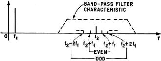
Another method, used by the Society of Motion Picture and Television Engineers,
also requires two input signals, one of which has 50 times the frequency and only
one-fourth the amplitude of the other. The output is put through a band-pass filter,
which filters out everything except the intermodulation terms. The latter are envelope-detected,
and then low-pass filtered. The distortion is defined as the modulation index of
the higher input frequency. With this method, both even- and odd-order non-linearities
are detected. The response to the even ones are the sidebands corresponding to f2
+ (2n-1)f1 and the response to the odd are the f22 ±
2nf1 sidebands. The bandwidth of the bandpass filter should be approximately
20 f1 to ensure passing all the sidebands.
With the conditions that e1/4 = e2, the intermodulation
distortion of a push-pull amplifier and a single-ended amplifier can be derived
from the Taylor series. They are shown in the table at the top of this column.
A serious drawback of this technique is that the envelope detection process is
nonlinear. If the signal amplitudes are low, as is often the case in transistor
circuits, envelope detection can add significantly to the distortion at the output.
Such circuits can be tested, however, if a wave analyzer - basically a selective
voltmeter - replaces the envelope detector. This procedure requires tuning to and
measuring all the spurious frequencies generated, and then computing the modulation
index. The results are very reliable, but the procedure is time-consuming and the
equipment is considerably more expensive than that used in the total harmonic distortion
method. And since all spurious frequencies must be measured, the upper cutoff frequency
of the system being tested must be 50 times greater than the lower cutoff frequency
to pass all the significant frequencies.
In fact, all of the methods discussed so far work only with broadband systems.
But there is one technique of intermodulation distortion measurement that is designed
specifically for such limited passband systems as intermediate-frequency amplifiers.
Again, two signals whose significant intermodulation products lie within the amplifier's
passband are applied to the system. In this technique, if e1 and e2
= e/2 then
IM(narrowband) =
This method detects only the odd-order terms of nonlinearity, since the sum of
the coefficients of the terms in the output closest to the test signal is odd. This
method is quite satisfactory in the case of i-f amplifiers, because only the odd
terms cause significant spurious responses. The equipment normally used is a wave
or spectrum analyzer.
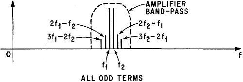
Odd Or Even
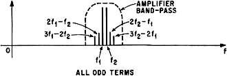
Two signals, close together, are used in the narrow band method
of distortion analysis. The amplifier under test has a narrow pass-band, and the
intermodulation terms measured are restricted to this band. As shown in the diagram
above, these terms are all odd.
To obtain complete distortion data, it is necessary, in most cases, to detect
both even and odd nonlinearities. Of the systems discussed, only total harmonic
distortion analysis and the SMPTE intermodulation methods have this capability.
A brief summary of a comparison between these two methods, made by W. J. Warren
and W. R. Hewlett2, is shown in the table on page 82. The ratios of intermodulation
to harmonic distortion (IM/HD) shown will hold true for any frequency-independent
system in a predictable manner. Both methods give the same information about the
coefficients of the power series describing the amplifier; the answers just differ
by a scale factor. Even so, intermodulation measurements are more difficult to make
and generally require more sophisticated equipment than total harmonic measurements.
Intermodulation measuring requires two test signals which have no prior interaction.
The distortion of these two signals does not have to be low, since their harmonics
will not usually cause any significant intermodulation products. Setting up a measurement
at one set of test frequencies is not difficult; but if measurements are required
at several different sets of frequencies, the procedure becomes very complicated
- especially if it is necessary to tune to each intermodulation term separately.
With the total harmonic distortion method however, both high and low frequency
response can be easily measured, since only one signal frequency need be changed.
This is useful when checking the effects of diminishing feedback gains at either
end of the frequency response characteristic or the effect of load capacitance at
the high-frequency end. In addition, the total harmonic distortion method requires
only that the system have a flat frequency response over a frequency deviation of
three to one, whereas the SMPTE method requires a flat response for a deviation
greater than 50 to one.
New Test Instrument
Since the nulling of the fundamental is normally the time-consuming portion of
total harmonic distortion measurement, great savings can be realized, especially
in production line testing with an analyzer which automatically rejects the fundamental.
The time saved is as much as 25 seconds of a 30-second measurement. With automatic
nulling, the accuracy of the null achieved is no longer a function of operator training,
manual dexterity or signal source frequency drift.
Automatic nulling circuitry in a new commercial wave analyzer, the H-P 333A and
334A, operates on the principle that the fundamental at either side of a Wien bridge
off null follows well-known phase relationships. In this instrument, phase-sensitive
feedback loops are employed which drive photo-cells in parallel with the resistances
on either side of the bridge. These loops reject the fundamental and are not critical
to adjust, since any imbalance on one side of the bridge is automatically compensated
for on the other. Imbalances on either side cause phase errors in the fundamental
which are in quadrature, so the phase-sensitive feedback loops are independent of
each other.
The analyzer will maintain a null even though there is a slow drift in the input
frequency. This ability to "pull" the null has opened the door to a number of applications
where the total harmonic distortion measurements were not readily applied in the
past. Among them are:
• Single-frequency production line testing of such components as integrated-circuit
amplifiers or transformers. As long as the long-term drift of the signal source
is less than ±1 %, a good null will always be achieved. Therefore, time-consuming
rebalancing operations at the test position are eliminated.
• Optimizing the performance of an oscillator. Here, any variation in the
parameters causes the frequency to shift slightly. The automatic nulling of the
analyzer allows the oscillator performance to be improved on a continuous basis,
rather than by relying on a point-to-point check, which may or may not find the
optimum point.
• Correcting distortion in signal generators which produce sine waves either
by mixing or by non-linear shaping. The small frequency shifts that occur in the
process would also cause the loss of the null if it were not for the automatic null
feature.
References
1. B.M. Oliver, "Distortion and intermodulation," Hewlett-Packard Co., Application
note 15.
2. W.J. Warren and W.R. Hewlett, "Analysis of intermodulation method of distortion
measurement," Proceedings of the IRE, p. 457-466, April, 1948.
The author
Charles R. Moore is a group leader at the research and development laboratories
of the Hewlett-Packard Company's Loveland division. He is a graduate of Princeton
University and earned his master's degree in electrical engineering at the University
of California.
Posted October 25, 2023
(updated from original
post on 10/22/2018)
|


")