|
December 1965 Electronics World
 Table of Contents
Wax nostalgic about and learn from the history of early electronics. See articles
from
Electronics World, published May 1959
- December 1971. All copyrights hereby acknowledged.
|
My first encounter with
a parametric amplifier was in the S-band search
radar system I worked on in the U.S.
Air Force. That was in the late 1970's - early 1980's, and the radar was an early
1960's era vacuum tube system with a few solid state upgrades. A silicon diode in
the receiver detector circuit, and a transistorized parametric amplifier in the
receiver front end are the only two that come to mind.* I remember the etch school
instructors making a big deal out of the parametric amplifier being so great because
it could actually improve the signal-to-noise ratio (SNR) of the received signal.
Even at the time, in my youthful ignorance, it seems too good to be true, but if
an ambassador of Uncle Sam - especially one wearing five times the number of stripes
on his sleeve that had I - then surely it must be so. Leap forward a decade in time
and I'm working at General Electric Aerospace Division in Utica, New York, freshly
endowed with a BSEE degree, and while researching a design for an airborne early
warning electronic countermeasures (ECM) system, a thought of that miraculous parametric
amplifier came to mind. There was no Internet back then, but the place had a very
nice technical library. Not much information was available, so I asked a couple
of the seasoned radar gurus about it, but none were particularly enthusiastic, so
I moved on. Over the years I have done some reading on parametric amplifiers and
never really found a good explanation of why they would have been deemed to have
effectively a negative noise figure (in decibels) - until I ran across this article
from a 1956 issue of Electronics World magazine.
* Interesting but not relevant to this discussion is that another modernization
upgrade from a decade earlier was an IF amplifier section that used
peanut vacuum tubes rather than the full-size tubes. Also, please contact me
if you have the schematics for the AN/MPN-13 or -14 radar.
Low-Noise R.F. Amplifiers
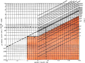
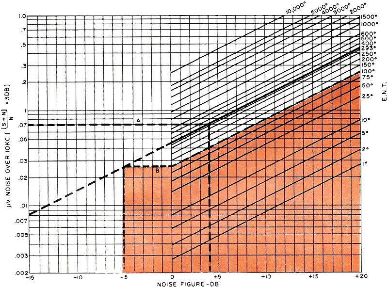
Fig. 1 - Comparison among conventional "microvolts sensitivity"
amplifier ratings, noise figure, and effective noise temperature (E.N.T.). Example
A shows conversion of microvolt sensitivity to noise figure at room temperature
(293°K). Example B shows conversion of 100°K E.N.T. to noise figure. Intersection
of 100° curve and 0 db point is extended to 293° line. The noise figure,
as read below, is -5 db.
By Jim Kyle
Special techniques including masers, parametric amplifiers, tunnel diodes, and
low-noise transistors are used to reduce receiver noise so that low-level signals
can be detected.
The absolute limitation on the usefulness of any communications system is the
electrical noise present in the system. Whether information is transmitted by wire
or radio wave, the signals suffer loss along the path from transmitter to receiver
- and when this loss makes the signal weaker than the inherent noise at the receiving
end of the system, the signal is lost for good.
Because of this, "signal-to-noise ratio" (usually abbreviated S/N) is used as
a key parameter of performance in such widely divergent areas of communication as
tape recording, telephone engineering, and radio.
And, also because of this, the object of virtually every technical improvement
in radio communications is to increase the signal-to-noise ratio.
The all-important S/N ratio can be increased in many ways. The most obvious way
is to increase transmitter power. If all other system parameters remain unchanged,
the S/N ratio will increase in a direct relationship as the transmitter power increases.
Conversely, a specified S/N ratio may be maintained at a greater range from the
transmitter.
However, the route of increasing power rapidly runs into limitations. One is
legal in nature - regulatory bodies limit the maximum power permitted in various
radio services; the other is physical-transmitting tubes capable of handling more
than a couple of million watts or so on a sustained basis simply aren't available.
So the engineer uses other techniques.
One of the favorites is the gain antenna. This can provide dramatic improvements
at first but then rapidly runs into physical limitations.
The technique which appears to offer the most promise at this time, and which
has already resulted in a tenfold or greater improvement in capabilities for some
types of communications, involves reducing the receiver's inherent noise.
Though the noise is present in every stage of the receiver, it is controlled
primarily by the amount of noise in the first r.f. amplifier stage alone. Only in
this stage is the raw incoming signal competing with the inherent noise; after this
stage, the signal has been amplified and will have a better chance of being stronger
than the noise of subsequent stages.
However, the inherent noise of the first r.f. stage is amplified just as much
as the signal, so that for any significant reduction in over-all receiver-noise
level, the noise level of the first r.f. amplifier must be reduced to the lowest
possible figure.
"Low-noise" r.f. amplifiers have been on the scene for decades. However, a number
of relatively recent developments have lent new dimensions of meaning to the almost
hackneyed phrase. Where formerly an r.f. amplifier with a 3-db noise figure was
considered good, amplifiers are now available which boast noise figures in the negative
db range when measured by conventional techniques.
Noise Figure
Before examining these newer techniques, it would be well to clarify some of
the terms used in discussing low-noise r.f. amplifiers. The foremost of these terms
is "noise figure."
"Noise figure" is a measurement of the relative amount of noise inherent in an
amplifier or a receiver. One of several definitions commonly accepted is that this
figure is the ratio of the S/N ratio existing at the input of the amplifier, to
the S/N ratio at the amplifier's output. Since no amplifier can actually improve
the signal-to-noise ratio of the original received signal, the noise figure obtained
by this approach will always be some value greater than unity.
Actually, two terms are in wide use in referring to receiver noise measurements,
and since the two are often used interchangeably, the resulting confusion is intense.
These terms are "noise figure" and "noise factor."
No clear-cut separation between their meanings exists. The consensus of usage
appears to be that noise factor is the ratio defined above, of input S/N to output
S/N, while noise figure is the same ratio but expressed in decibels rather than
as a dimensionless ratio. Thus, a "perfect" amplifier would have a noise factor
of 1, or a noise figure of 0 db. Since the important thing about noise is power
rather than voltage or current, the ratios convert to db by the power-decibel equation;
a ratio of 2 equals 3 db.
Both noise factor and noise figure must be dealt with, Since the equations used
in determining noise levels and their effects most usually cannot employ logarithmic
numbers, while the pure ratio expressed by the noise factor is not nearly so meaningful
when examining a complete system.
The major reason for employing noise figure at all as a measure of amplifier
performance is that it is a more direct indicator of actual performance than is
a "microvolt-sensitivity" rating. The amount (measured in millimicrovolts) of noise
present in an amplifier depends to a large degree upon the bandwidth of the amplifier.
Thus, to use microvolt-sensitivity ratings, the noise bandwidth of the amplifier
must also be known. However, due to the manner in which noise figure is measured,
the bandwidth is almost immaterial; the noise figure yields a direct indication
of the amount by which the S/N ratio of the incoming signal will be degraded by
the amplifier's inherent noise.
It cannot be overemphasized that noise figure alone is not an adequate measurement.
A straight piece of hookup wire a couple of inches long has a noise figure of 0
db. However, it is useless as an amplifier. When using noise figure as the parameter
of performance, gain must also be specified.
The fact that several of the newer devices yield noise figures in the negative
db range (noise factors less than unity) implies better-than-perfect performance.
This is not so, and the newer devices do not improve the S/N ratio of the incoming
signal. The apparent contradiction is due to the fact that the noise-figure equations
usually employed to calibrate measuring instruments include an assumption that all
parts of the amplifier are effectively at room temperature (293° K is the usual
assumed temperature), since the amount of noise present depends largely upon the
temperature of the components. Noise of the newer devices is so low that the effective
temperature is far lower than that assumed, yielding "incorrect" results (which
are, however, meaningful because they have consistent error since a "-4 db" amplifier
is still 10 db better than a "+6 db" amplifier).
To escape this built-in error, neither noise factor nor noise figure is used
to evaluate many of the newer devices. Instead, "effective noise temperature" is
employed as the parameter. Although not directly interchangeable with "noise figure,"
it can be roughly compared. Fig. 1 shows such a comparison among microvolt ratings
(10-kc. bandwidth), noise figure, and effective noise temperature.
Maser
Probably the most spectacular of the newer devices, as well as the one which
has received the widest publicity, is the maser. This is a device for microwave
amplification by stimulated emission of radiation and operates on principles more
closely akin to nuclear physics than to conventional radio circuitry.
Briefly, the operating principle is this. Certain materials have their molecules
arranged in such a manner that some electrons in the atomic shell can be "lifted"
to a higher-than-normal energy level by interaction with a magnetic field. When
the lifted electrons absorb an amount of energy determined both by the material
and by the strength of the magnetic field, they "fall back" to the original level,
and in so doing release their stored energy in the form of radiation. The frequency
at which this radiation is emitted is determined primarily by the magnetic-field
strength.
In the maser, things are arranged in such a way that the energy absorbed by the
electrons is provided by a local "pump" oscillator, while the energy released by
radiation is applied to the r.f. signal instead. Thus, energy is added to the signal,
and this is (by definition) amplification.
Actually, two basically different types of solid-state masers are in use. The
one described most frequently is the "cavity maser" in which the active material
(usually a ruby crystal) is placed in a resonant cavity, tuned so as to be resonant
at both the pump and signal frequencies. The one more widely used, however, is the
"traveling-wave maser" in which the active material is placed in a waveguide to
form a slow-wave structure, so that the r.f. signal will be exposed to the maser
action for a longer period of time, allowing the maximum possible field interaction
to take place.
Both the cavity and the traveling-wave masers are capable of extremely low-noise
operation. Effective noise temperature of either type of maser can approach 1°K,
which corresponds to a noise figure of between -15 and -25 db (depending upon which
reference book is consulted for the conversion factors and techniques).
The cavity maser, however, has rather limited bandwidth and so is dropping out
of general use. The traveling-wave maser's bandwidth is much greater. The Telestar
satellite uses a traveling-wave maser, with signal-to-noise ratio better than 70
db over a 30-mc. bandwidth, operating with a received signal power of only about
one-millionth of one micro-\watt. This calculates to a "noise figure" of -7.8 db.
Both types of masers are limited to the microwave region and above; they do not
function successfully below about 1 gc. Maser action, in addition, occurs only at
exceptionally low temperatures. Operating units are cooled with liquid nitrogen
or liquid helium. Hence, masers are physically rather complex devices as well.
Thus, while the maser appears to be the nearest thing to a perfect amplifier
yet developed, it is too complex to enjoy wide use with portable equipment. In addition,
it offers no help at all in the lower u.h.f. region and below.
Parametric Amplification
One of the most popular of the other new techniques is that of parametric amplification.
Like the maser, it utilizes a local pump oscillator, and power is transferred from
the pump to the signal. However, unlike the maser, the parametric amplifier operates
at room temperature and requires no exotic precious-gem components.
The principles of parametric amplification are best explained by use of an analogy.
Consider a conventional variable capacitor electrically in series with a transmission
line and mechanically coupled to a high-speed electric motor. As the motor rotates
the capacitor shaft, the capacitance varies from maximum to minimum and back again.
If this capacitor is connected in series with a transmission line carrying a
signal, at the instant the capacitor shaft is turned to maximum-capacitance position,
the voltage across the line will charge the capacitor. As the shaft rotates toward
lower capacitance positions, the charge on the capacitor must remain constant Since
it has no place to be dissipated. However, the capacitance is decreasing, and since
the charge remains constant the voltage across the capacitor must increase to compensate.
It is true that if the capacitor is charged at minimum capacitance, its voltage
will decrease as the shaft turns toward higher capacitance positions. However, if
the rate of capacitance change is much faster than the rate of change of voltage
in the signal, the net result will be a transfer of energy from the rotational force
driving the capacitor to the signal-output channel, and amplification will occur.
Since no resistances are involved, the action is theoretically free from all noise.
This electro-mechanical version cannot be made to operate at useful frequencies
because the capacitor cannot be turned rapidly enough. By substituting a voltage-variable
capacitor for the mechanically variable one and applying an a.c. voltage to the
capacitor instead of using a motor, the amplifier can be made to function well into
the microwave region.

Fig. 2 - Basic circuit of a low-noise parametric amplifier.

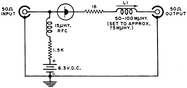
Fig. 3 - Tunnel diode r.f. amplifier providing 32 db gain at
100 mc. having a symmetrical bandwidth of 20 mc. L1 controls both gain and bandwidth.
The calculated noise figure is 8 db.
The circuit of such an amplifier appears in Fig. 2. Many variations are possible,
and most of them have been used at one time or another. The first working paramp
(parametric amplifier) used a single resonant cavity, with pump frequency chosen
to be twice signal frequency so that the cavity could be made simultaneously resonant
at pump, signal, and idler frequencies. Later models have used individually tuned
tank circuits and have combined pump with idler, signal with pump, and signal with
idler, to obtain two-tank operation.
This "idler" frequency which was mentioned in the preceding paragraph is unique
to parametric amplification. It has many of the characteristics of the "sum" or
"difference" frequencies found in mixer circuits, but in the paramp it is not actually
used. Although unused, it cannot be ignored, however. Unless it is properly disposed
of through a tank circuit that allows it to circulate and keeps it away from the
rest of the circuit, no amplification will be obtained.
Noise performance of the paramp depends primarily upon the ratio of pump frequency
to signal frequency. The greater this ratio, the lower the noise. Some configurations
of paramps appear to have no lower noise limit (could this ratio be raised to a
figure approaching infinity), while others seem to reach a "floor" in the neighborhood
of "-1 db" noise figures. In terms of effective noise temperature, performance in
the 20°K region has been reported at a signal frequency of 6 gc., with the paramp
refrigerated to a temperature of 90°K. With room-temperature components, 55°K effective
noise temperatures have been recorded at 6 gc. Noise performance appears to be relatively
independent of frequency between 400 mc. and 6 gc. where the majority of work with
paramps has occurred.
In comparison with the maser, the paramp has the advantage of greater simplicity
but suffers the disadvantage of slightly poorer performance. Its commercial and
military applications are primarily in the area of portable and mobile equipment;
fixed stations which are not intended to be moved at any time tend to use the maser
where possible because of its better performance. Complexity of operation is about
equal for both types of amplifiers.
Tunnel Diodes
A simpler approach to low-noise amplification than either of the methods already
discussed and which yields performance approaching but not equaling the maser and
the paramp, involves the Esaki or tunnel diode.
This device is a specially treated semiconductor diode which exhibits a "quantum
mechanical tunneling" effect and which, under proper circuit conditions, is effectively
a negative resistance.
By connecting this negative resistance into a tuned circuit low-noise amplification
may be obtained.
A 100-mc. tunnel-diode amplifier circuit, designed to be inserted in a 50-ohm
transmission line, is shown in Fig. 3. This circuit was intended for high gain over
a wide bandwidth, rather than for lowest noise, and so the designers (G-E) did not
specify noise performance. Calculated noise figure from published constants appears
to be approximately 8 db.
Lower noise figure would be obtained by reducing the source impedance seen by
the amplifier (through tuned-transformer techniques) and by reducing current flow,
but this would require complete redesign to avoid circuit oscillation.
The tunnel-diode amplifier is the simplest of all low-noise r.f. amplifier circuits,
both in arrangement of parts and in the number of components, but suffers one serious
disadvantage at the present state of the art. The diode itself is capable of amplification
at an infinite number of frequencies simultaneously and can also oscillate at a
near-infinite number of frequencies while amplifying at all the rest. This makes
the stabilization of such an amplifier a most tedious process. Regardless of the
frequency at which a tunnel-diode amplifier is to operate, u.h.f. construction facilities
must be employed in order to suppress parasitic oscillations.
Despite this disadvantage, designers are presently conducting intensive study
of the tunnel diode for use in u.h.f.-TV circuitry; it can be expected to appear
in mass-produced consumer equipment within the next few years.
Transistors & Special Tubes
All of the low-noise techniques discussed heretofore have involved either radically
different concepts, or specialized new components, or both. However, transistors
and vacuum tubes have also made recent strides forward in low-noise performance
to the point that the more exotic techniques are proving to be less and less necessary
for all but the most exacting applications.
For instance, transistors are now in production which have guaranteed maximum
noise figure of 4.5 db at signal frequencies up to 500 mc., with noise figure of
2 db or less at lower frequencies. This, while not as spectacular as the performance
of the maser or the paramp, still represents a notable achievement when compared
with the low-noise amplifiers of only a few years ago.
Circuitry for low-noise amplifiers using these newer transistors is virtually
identical to established, standard transistor r.f. amplifier circuits and is not
shown here.
One of the best performers among transistors in the noise arena is the 2N2857,
produced by RCA and by Kmc Semiconductor Corporation. This one is guaranteed to
have a noise figure below 4.5 db at 500 mc. and below 2 db at 200 mc. A runner-up
is the development type number A1243 from Amperex Electronic Corp., with 9-db noise
figure at 1 gc., 5 db at 500 mc., and 3.5 db at 70 mc. The 2N2495 from Amperex exhibits
a 2-db noise figure in the range from 150 kc. up to 25 mc., increasing to 5 db at
200 mc. Similar low-noise transistors are also produced by Philco, Sprague, and
others.
Advances in noise performance of vacuum tubes are due primarily to new manufacturing
techniques developed by a number of firms which allow closer control of tube characteristics
and permit virtually microscopic tube structures.
Most widely publicized of these advances is probably RCA's nuvistor, which has
been thoroughly described in the electronic press since its introduction. This thimble-sized
ceramic-and-metal tube features coaxial construction with multiple supports for
each element. The resulting structure is so rigid that the tubes are almost immune
to damage.
Most widely known of the nuvistors are the types 6CW4 and 6DS4, both triodes
intended for v.h.f. amplifier service in TV tuners. However, many other types are
also available under industrial (four-digit) type numbers. Among these are the 8058,
which features double-ended construction and automatic grid grounding, and the 8056,
a low-plate-voltage triode. The construction of the 8058 is especially designed
for u.h.f. use, and it may be employed well into the microwaves, thus extending
the advantages of nuvistors into u.h.f. (lead inductance limits the 6CW4 and 6DS4
above 200 mc.).
The nuvistor is not, however, the only new type of tubes providing low-noise
performance. An equally important advance is that known as "frame-grid" construction,
which apparently originated with Philips of the Netherlands and is now employed
by most major tube manufacturers the world over for certain types of tubes.
The frame grid is a special construction technique for maintaining absolute precision
in the spacing of the grid wire which, in turn, allows the tube to be designed for
much greater transconductance. This leads to low noise.
One of the first of the frame-grid tubes was the type 6ES8, which can be substituted
for the 6BQ7 series of cascode-design tubes in most existing r.f. amplifiers with
slight modification of supply voltages and in some cases of neutralization networks;
it provides a dramatic reduction in the receiver noise.
Later models include the 6HA5 single triode and the 7788 pentode. The 7788 is
unique in that, although a pentode, it provided lower noise than most high-quality
triodes. When triode-connected, its noise figure is virtually the lowest obtainable
with vacuum tubes, being bettered only by the next group of vacuum tubes to be discussed.
Both frame-grid and nuvistor tubes are classified as normal receiving types.
Another type of low-noise tube, the ceramic planar triode, falls into the special-purpose
Category. Used mostly in critical military and space applications, this type of
tube offers the best noise performance available from conventional vacuum-tube circuitry.
These tubes physically resemble small shirt buttons more than they do vacuum
tubes. Designed especially for grounded-grid circuits, they are constructed specifically
to be inserted in coaxial-line cavities and are intended for the u.h.f. and lower
microwave-frequency ranges. The cathode connection is at one end (with the heater
connections coaxial to it) and the grid is in the middle, with the plate connection
at the other end.
As the name implies, construction of these tubes is planar rather than coaxial.
The cathode is a flat surface, with the grid parallel to it and only a few thousandths
of an inch away. The plate is a third plane surface, also parallel.
Noise figures of these tubes range from 3 to 8 db depending upon frequency and
tube type. This surpasses both the frame-grid tube and the nuvistor in the upper
u.h.f. and lower microwave regions. At lower frequencies, noise figure of the planar
triode drops toward the vanishing point.
Major disadvantages of the ceramic planar triode are its cost and its low availability.
Posted November 25, 2022
|