|
July 1963 Electronics World
 Table of Contents
Wax nostalgic about and learn from the history of early electronics. See articles
from
Electronics World, published May 1959
- December 1971. All copyrights hereby acknowledged.
|
When you read this article's title,
I doubt you immediately thought it would be about a vacuum tube circuit, or even one that
uses discrete transistors to implement the circuit. Rather you most likely though it would
be about an integrated circuit (IC). Operational amplifiers (opamp) are building blocks characterized
(ideally) by their infinite input impedance, zero output impedance, infinite open-loop bandwidth
and gain, zero input offset voltage, amongst other defined parameters. The first commercially
produced integrated circuit (IC) opamp came to market in 1964 via Fairchild Semiconductor
(the µA702,
brainchild of Bob Widlar).
That was the year after this article was printed, and it's interesting to note that the schematic
symbol had already been established prior to IC versions. Vacuum tube opamps were common in
control systems for radar antenna controls and big guns on ships in World War II.
The Operational Amplifier
By Jack E. Frecker / Applied Research Lab., University of Arizona
Part 1 / These circuits are widely employed in industrial test equipment and analog computers.
Theory of amplifier along with design and construction of a unit are covered.
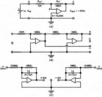
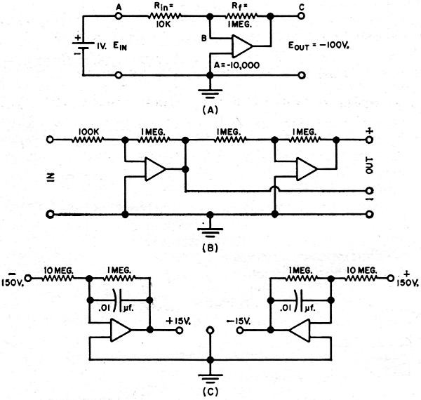
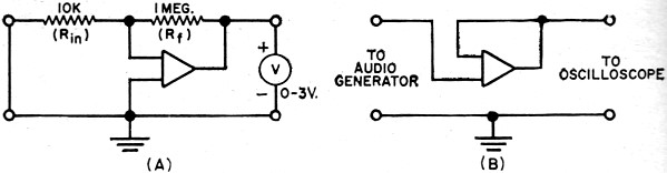
Fig. 1. (A) Typical use for operational amplifier. (B) An audio phase inverter
with a gain of 10. (C) Method of using operational amplifiers as an extremely well-regulated
supply.
The operational amplifier was originally invented to perform precise mathematical operations
in electronic analog computers. Yet some of its most fascinating uses are in other than computing
applications. How would you like one device that could be used, simply by connecting a few
external parts, as an amplifier, an oscillator, a voltmeter calibrator, a regulated power
supply, a precision oscilloscope sweep generator, a capacitance bridge, and even as an analog
computer. This is the operational amplifier.
Its uses are literally unlimited. The sheer act of building and using operational amplifiers
could no doubt cause the reader to discover some new applications. This article will acquaint
the reader with the operational amplifier, show the design and construction of a two-amplifier
unit, and describe in detail several representative uses of same.
Basic Concepts
Just what is the operational amplifier? How is it different from any other amplifier? First
of all, it is a feedback amplifier for which the user supplies the feedback components. These
components, incidentally, may be resistive, reactive, or non-linear. It is capable of any
amount of feedback. One usage that will be described later involves reducing the amplifier
open-loop gain (gain without feedback) from several million to a gain of 1/10 by means of
feedback. An ordinary audio amplifier would break into oscillation or motorboating if this
were tried. Such operation is possible with an operational amplifier because of two of its
characteristics. It is direct coupled (this makes motorboating impossible), and its gain is
rolled off to less than unity before the necessary phase shift to sustain oscillations takes
place. Second, its characteristics are determined to the greatest degree possible by the feedback
components. If you have ever tried to calculate feedback components for an ordinary amplifier
you will know that amplifier gain, output impedance, and various stability criteria enter
into the calculations. For the operational amplifier the calculations simply involve the ratio
two external impedances.
Basically, the operational amplifier is a direct-coupled amplifier, and with the input
grounded the output is at zero volts d.c. in respect to ground. Its gain is exceedingly high,
1000 to 15,000 being typical for simple devices and gains to one billion being found in laboratory
units. Its output impedance is quite low by nature and, with feedback, it is further reduced
to where it becomes negligible.
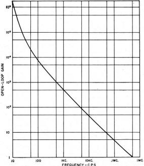
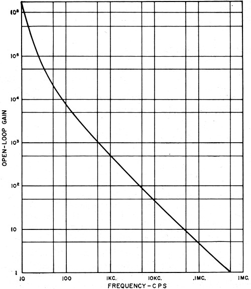
Fig. 2. Plot of amplifier gain vs frequency is close to ideal.
A typical application is that of Fig. 1A. An amplifier with a gain of -10,000 is shown
for illustration, the minus sign denoting a phase inversion between the input, point A, and
the output, point C. The external feedback components are resistors Rin and Rf.
With the +1-volt battery connected to the input, the output will start to go highly negative.
This output will be fed back to the summing junction, point B, in a degenerative manner, tending
to prevent the output from going negative. The circuit will reach a state of equilibrium with
the output at about -100 volts, which is -100 times the input voltage, or equal to the ratio
-Rf/Rin. It can be shown that if the amplifier open-loop gain were infinite
the system gain would simply be -Rf/Rin. And it can also be shown that
if the amplifier gain were only (-Rf/Rin) x 100, the system gain would
be within one per-cent of the ratio -Rf/Rin. Similarly, if the output
impedance of the amplifier without feedback were about 500 ohms and the gain reduced by a
factor of 100 by feedback, the output impedance would also be reduced by more than a factor
of 100, to less than five ohms. By the same token, amplifier noise and distortion are reduced
by similar amounts.
Another point to remember about the operational amplifier is the nature of the summing
junction, point B of Fig. 1A. With +1 volt at the input, point A, and -100 volts at the output,
the voltage at the summing junction will be -1001/-10,000 or 0.01 volt. This point behaves
as a very low resistance to ground, and since it does so we can define the input impedance
to the system as simply the value of Rin, or 10,000 ohms in Fig. 1A.
Figs. 1B and 1C are very practical applications of the above principles and both are possible
with the unit to be described. Fig. 1B is an audio phase inverter with a gain of 10. The first
amplifier provides a gain of 10 and furnishes the negative or inverted output. It also drives
the second amplifier which is connected as a unity-gain inverter. This amplifier re-inverts
the first amplifier's output to provide a positive or non-inverted output. The circuit is
useful for driving audio power amplifiers. It could provide a balanced low-impedance output
for a single-ended audio generator, or it could drive the deflection plates of an oscilloscope
which has no d.c. amplifier.
Fig. 1C is an extremely well-regulated electronic power supply which furnishes plus and
minus 15 volts at 4 ma. each for experimental transistor circuits. The first amplifier amplifies
the -150·volt reference source by - (1/10) to provide +15 volts. The second amplifier amplifies
the +150·volt reference source by -(1/10) to provide -15 volts. The two capacitors provide
a.c. feedback which is employed in order to give the circuit a very low output impedance.
Two-Amplifier Unit
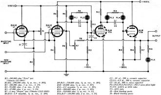
Fig. 3. Schematic diagram of one of two identical operational amplifiers
that are employed in the author's design.
After much planning and experimenting, it was decided to design and construct two operational
amplifiers within a single housing, their power supply, a 6BJ7 triple diode for auxiliary
functions requiring diodes, and plus and minus 1.50-volt reference voltages. Two amplifiers
are far more useful than one, but three would have complicated the power-supply requirements
and made the unit quite costly.
The requirements of an operational amplifier are that with the inputs grounded, the output
should be at zero volts d.c. with respect to ground; that the gain be quite high; and that
the output impedance without feedback be fairly low. In addition, the unit must be direct
coupled and its open-loop gain must be rolled off to less than unity before unwanted amplifier
phase shift reaches 180 degrees. These last two requirements make it possible to use any amount
of feedback without danger of oscillation. Another requirement is that d.c. drift be quite
low.
The following discussion of amplifier No.1 (see Fig. 3), composed of V1, V2, and V3, also
applies to amplifier No.2 which is identical.
In the circuit, V1 and V2 comprise a differential amplifier. (Such an amplifier consists
of a cathode-coupled pair with output taken at the second stage. It takes its name from the
fact that with inputs applied to both grids simultaneously, the output responds approximately
to the difference between the two input signals.) This circuit is invariably used as the first
stage of an operational amplifier because any change in heater voltage, the major cause of
drift, will affect both tubes in an equal and opposite fashion, tending to cancel out the
effect of drift. In addition, the existence of a differential input permits many applications
of the unit which would not otherwise be possible.
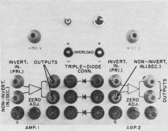
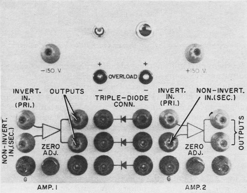
Front-panel view showing all interconnecting binding posts.
The amplifier has two inputs. The grid of V1 is the primary input. There is phase inversion
between this input and the output. This input is the upper one used in all the diagrams. The
grid of V2 is the secondary input and is the lower one in the drawings. There is no phase
inversion between this input and the output.
V2 could have been coupled to V3A by means of a 2.2-megohm resistor from V2 plate to V3A
grid, and then another 2.2-megohm resistor from this grid to -150 volts. However, this would
have resulted in 6-db attenuation of the signal. A better way is the use of neon lamps. Neon
lamps work much like gas regulator tubes; that is, the d.c. voltage drop across them remains
nearly constant with a fairly wide variation of current flow through them. The plate voltage
of V2 is about +160 volts. This is dropped 55 volts by PL1, 50 volts by R9, and 55 volts by
PL2. Any amplified signal at the V2 plate will be coupled without loss by PL1 and PL2 and
will be attenuated only slightly by R9. R11 provides the current to keep the lamps lit, about
70 μa.
R1 is the amplifier zero-adjust control. By varying the screen voltage of V1, R1 adjusts
the d.c. operating point of the amplifier and is used to set the amplifier output to zero
volts d.c. with both inputs grounded.
V3A is a d.c. amplifier with a gain of -200. R10 limits the screen current of this tube
to a value safe for the tube under amplifier overload conditions. This stage drives cathode-follower
V3B which has an output impedance of about 400 ohms. The neon light at the output terminal
glows when the output goes plus or minus 70 volts and indicates an overload.
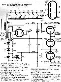
Fig. 4. Single power supply used for both operational amplifiers.
R7 and R8 are connected from the output to the screen of V2 and provide positive feedback
to increase the amplifier gain from about 15,000 to a value approaching infinity at d.c. C3
provides negative feedback in V3A at frequencies above d.c. and is used to reduce amplifier
gain, at a rate of 6 db per octave, to less than unity before a total of 180 degrees additional
phase shift in both stages takes place. As this capacitor is for all practical purposes connected
from plate to grid instead of plate to ground its effective capacity is multiplied by the
gain of the stage. Its value was selected by trial and error and is just large enough to give
the amplifier a damping factor of 0.5 to a square-wave input. A plot of amplifier gain versus
frequency is shown in Fig. 2. This plot is close to the idealized curve for operational amplifiers.
The amplifier requires regulated d.c. voltages to prevent drift. The power supply is a
conventional gas-tube shunt-regulated type. Its outputs are +150 volts, +300 volts, and -150
volts, all regulated, and -300 volts unregulated (Fig. 4).
Construction Details
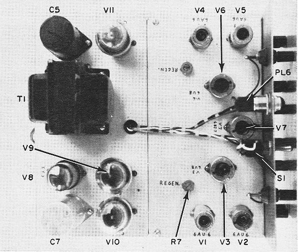
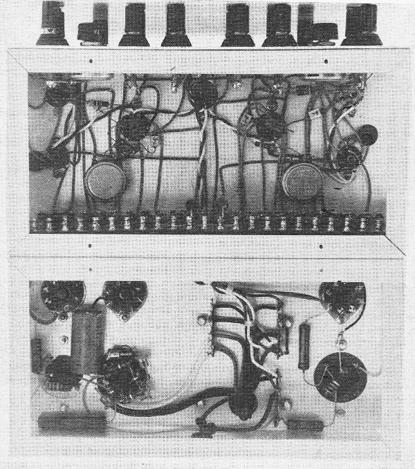
The unit is constructed on two 9 1/2" x 5" X 3" aluminum chassis bolted together with the
power supply in the rear and the two amplifiers and the 6BJ7 triple diode in front. This two-chassis
arrangement provides excellent shielding from 60-cycle hum. C5 and C7 are can-type electrolytic
capacitors. The can of C5 must be insulated from ground and should be covered with electrical
tape to prevent accidental shock to the user. Most of the amplifier components are mounted
on a terminal board. Although the zero-adjust potentiometers are on the front panel, they
could very well have been mounted on the chassis surface and have been of the screwdriver-adjust
type as they rarely have to be touched.
All of the amplifier input and output terminals, the triple-diode terminals, and the plus
and minus 150-volt reference terminals are brought to the front panel on three-way binding
posts. It is on these binding posts that the external feedback components and other external
circuitry components are mounted during use. The black binding posts under the amplifier output
terminals are unused.

Top view showing the two-chassis construction used by author.

Fig. 5. (A) Connections used to check for reduced line-voltage operation.
(B) Setup to check for distortion less unity gain.
The "on-off" switch, pilot light, and overload indicator neons are also on the front panel.
The neon lights are inserted in 1/4" grommets and secured with rubber cement. They should
be mounted with one terminal directly above the other. The upper terminal is grounded and
the lower terminal is connected through the 910,000-ohm resistor to the amplifier output.
When the upper electrode glows, a positive overload is indicated and when the lower electrode
glows a negative overload is indicated. After the front panel is cut, drilled, and punched
and before it is mounted, it should be sprayed with gray paint. Then all of the symbols are
marked on it with India ink and a final coat of clear acrylic spray is applied to secure the
India ink markings. The rest of the construction details are obvious from the photos.
Adjustment and Testing
After the unit is completed and the wiring checked for errors, it may be tested as follows.
First insert all power-supply tubes and turn the unit on. All three regulator tubes should
light. Then plug in the three tubes of amplifier No.1 and ground the two inputs. After a minute's
warm up, it should be possible to balance the amplifier. Set R7 to maximum resistance. Turn
the zero-adjust control, R1, slowly from one extreme to the other. At some point the overload
indicator will change from a positive indication to a negative indication. The point where
this change takes place is the correct setting. If this condition cannot be met, the two 6AU6
tubes are probably not sufficiently well matched for this application. Try substituting other
6AU6 tubes until a pair is found that will permit balancing.
Then connect the amplifier as shown in Fig. 5A. Offset the zero-adjust control sufficiently
to cause a mid-scale reading on the voltmeter. Note this reading. Then decrease the line voltage
by 10 per-cent by switching a 25-ohm, 5-watt resistor in series with the power line. The voltmeter
reading will slowly change to some new value as the tube heaters cool off. This change in
the voltmeter reading should be less than one-half of a volt. If it is greater than half a
volt, try different 6AU6 tubes until a sufficiently well matched pair is found to meet this
specification. Then restore line voltage to normal.
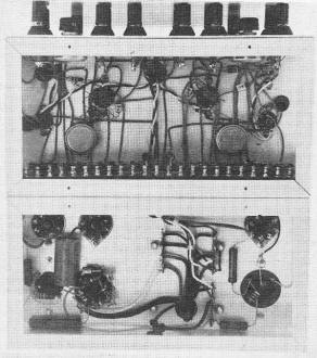
Bottom-chassis view of amplifier. Note use of terminal board.
To set the regeneration potentiometer, R7, connect the amplifier as shown in Fig. 5A, only
with Rf = 10 megohms and Rin = 100 ohms. Use a direct-coupled oscilloscope
instead of the meter. Slowly turn the zero-adjust control back and forth to cause the amplifier
output to go into its upper and lower limits, and steadily decrease the resistance of the
regeneration potentiometer R7. The zero-adjust control will get more and more sensitive. Soon
a point will be reached where the amplifier output suddenly switches from one voltage to another
and cannot be set to any value in between. Back off the regeneration potentiometer slightly
from this position. This is now the correct setting.
Next connect the amplifier as shown in Fig. 5B. The amplifier should provide unity gain
to the signal coming from the audio generator and the output should be free from any distortion
or parasitic oscillations from the lowest possible frequency to 100 kc.
Repeat all the previous test procedures for amplifier No.2 and plug in the 6BJ7 tube. When
tests are completed the unit is ready for use.
Next month, some sophisticated uses of the operational amplifier unit will be presented,
including a voltmeter calibrator, frequency-sensitive feedback circuits, oscillators, a capacitance
bridge, multi vibrators, and others.
(Concluded Next Month)
Posted January 26, 2017
|