|
|||||||||||||
 |
|||||||||||||
The Operational Amplifier
|
|||||||||||||
There is no such thing as too many introductory articles on operational amplifiers (opamps). Of course, when this story was written for Electronics World back in 1967, opamps were relatively new to the scene. Prior to the advent of opamps, circuit design for controllers, filter, comparators, isolators, and just plain old amplification was much more involved. Opamps suddenly allowed designers to not worry as much about biasing, variations in power supply voltages, and other annoyances, and instead focus on function. Even from the very beginning with the μa741 operational amplifier, the parameters came close to those of an ideal device: infinite input impedance, zero output impedance, perfect isolation between ports, and infinite bandwidth. OK, the bandwidth spec was more constrained compared to the other three, but still, with frequencies being what they were compared to today, it was close enough. Opamps allowed engineers to design with the simplicity of LaPlace equations. The Operational Amplifier - Circuits & Applications By Donald E. Lancaster
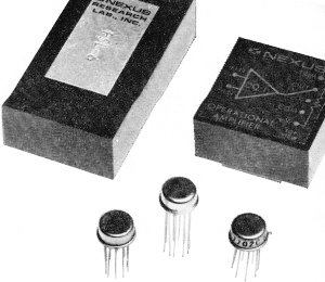
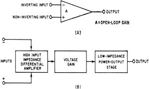
Typical modular package and TO-5 style IC operational amplifiers. These highly versatile controllable-gain modular or integrated-circuit packages have been used in computer and military circuits. New price and size reductions have opened commercial and consumer markets. Here are complete details on what is available and how the devices are used. Once exclusively the mainstay of the analog-computer field, operational amplifiers are now finding diverse uses throughout the rest of the electronics industry. An operational amplifier is basically a high-gain, d.c.-coupled bipolar amplifier, usually featuring a high input impedance and a low output impedance. Its inherent utility lies in its ability to have its gain and response precisely controlled by external resistors and capacitors. Since resistors and capacitors are passive elements, there is very little problem keeping the gain and circuit response stable and independent of temperature, supply variations, or changes in gain of the op amp itself. Just how these resistors and capacitors are arranged determines exactly what the operational amplifier will do. In essence, an op amp provides "instant gain" that may be used for practically any circuit from a.c., d.c., and r.f. amplifiers, to precision waveform generators, to high- "Q" inductorless filters, to mathematical problem solvers. Op amps used to be quite expensive, but many of today's integrated circuit versions now range from $6 to $20 each and less in quantity. Due to price breaks that have occurred very recently, the same benefits now available to the analog computer, industrial, and military markets are now extended to commercial and consumer circuits. One obvious application will be in hi-fi preamps where a single integrated circuit can replace the bulk of the low-level transistor circuitry normally used. Fig. 1A shows the op-amp symbol. An op amp has two high-impedance inputs, the inverting input and the non-inverting input, as indicated by a "-" or a "+" on the input side of the amplifier. The inverting input is out-of-phase with the output, while the non-inverting input is in-phase with the output. The amplifier has an open-loop gain A, which may range from several thousand to several million.
Fig. 1. (A) Op-amp symbol. (B) Block diagram of typical op amp.
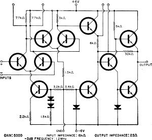
Fig. 2. Characteristics of the Fairchild μA702C. Price: $9.00.
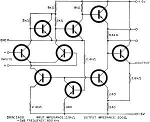
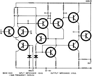
Fig. 3. Characteristics of Motorola's MC1430. Price: $12.00.
Fig. 4. The RCA CA3030 operational amplifier. Unlabeled terminals are used for frequency-compensation. Price: $7.50. Note that the prices given here and above are for single-unit quantities and these prices are subject to change. On closer inspection, we see three distinct parts to any operational amplifier's internal circuitry, as shown in Fig. 1B. A high-input-impedance differential amplifier forms the first stage, with the inverting input going to one side and the non-inverting input the other. The purpose of this stage is to allow the inputs to differentially drive the circuit and also to provide a high input impedance. There are several possibilities for this input stage. If an ordinary matched pair of transistors (or the integrated circuit equivalent) is used, an input impedance from 10,000 to 100,000 ohms will result, combined with low drift, low cost, and wide bandwidth. By using four transistors in a differential Darlington configuration, the input impedance may be nearly one megohm. Drift and circuit cost are traded for this benefit. Field-effect transistors are sometimes used, yielding input impedances of 100 megohms, but often with limited bandwidths. FET integrated-circuit operational amplifiers are not yet available, limiting this technique to the modular-style package at present. One or two novel techniques allow extreme input impedances, but presently at very high cost. One approach is to use MOS transistors with their 1013-ohm input impedance; a second is to use a varactor diode parametric amplifier arrangement on the input. The input differential amplifier is followed by ordinary voltage-gain stages, designed to bring the total voltage gain up to a very high value. Terminals are usually brought out of the voltage-gain stage to allow the frequency and phase response of the op amp to be tailored for special applications. This is usually done by adding external resistors and capacitors to these terminals. Since an operational amplifier is bipolar, the output can swing either positive or negative with respect to ground. A dual power-supply system, one negative and one positive, is required. The final op-amp stage is a low-impedance power-output stage, which may take the form of a single emitter-follower, a push-pull emitter-follower, or a class-B power stage. This final circuit serves to make the output loading and the over-all gain and frequency response independent. It also provides a useful level of output power. THE MATH BEHIND THE OP AMP The gain of an operational-amplifier circuit is always chosen be much less than the open-loop gain of the amplifier itself. This allows the circuit response to be precisely determined by the external feedback and input network impedances. Feedback is almost ways applied to the inverting (-) input. This is negative feedback for any change in output tries to produce an opposing change in the input. The feedback and input network impedances are normally chosen such that they are much larger than the op amp's output impedance, much smaller than the op amp's input impedance, and such that the gain they require for proper operation is much less than the amp's gain. If these assumptions are met, the ratio of input to output voltage (the gain of the circuit) will be given by: Circuit Gain =
For instance, the op-amp circuit of Fig. 5B has an input impedance of 1000 ohms and a feedback impedance of 10,000 ohms Its gain will be - 10k/1k = - 10. Any of the op amps of Figs. 2, 3, or 4 may be used for this circuit. Some circuit analysis will show that the inverting input is always very near ground potential, and this point is then called a virtual ground insofar as the input signals and output feedback are concerned. Thus the input impedance to the circuit will exactly equal the input network impedance. When capacitors are used in the networks, the phase relationships between current and voltage must be taken into account. These differences in phase allow such operations as differentiation, integration, and active network synthesis. But isn't an op amp a d.c. amplifier and don't d.c. amplifiers drift and have to be chopper-stabilized or otherwise compensated? This certainly used to be true of all amplifiers, but today such techniques are reserved for extremely critical circuits. The reasons for this lie in the input differential stage. It is now very easy to get an integrated circuit differential amplifier stage to track within a millivolt or so over a wide temperature range. This is due to the identical geometry, composition, and temperature of the input transistors. Matched pairs of ordinary transistors can track within a few millivolts with careful selection. FET's offer still drift performance, as one bias point may be selected that is drift-free with respect to temperature over a very wide range. Thus, chopper-stabilized systems are rarely considered today for most op-amp applications. There are three basic op-amp packages available today. The first type consists of specialized units used only for precision analog computation and critical instrumentation circuits. These are priced into the hundreds and even thousands of dollars for each category, and are not considered here. The second type is the modular package, and usually consists of a black plug-in epoxy shell an inch or two on a side. Special sockets are available to accommodate the many pins that protrude out the case bottom. The third package style uses the integrated circuit. Here the entire op amp is housed in a flat pack, in-line epoxy, or TO-5 style package. (See lead photograph.)
Table 1. Comparison between integrated operational amplifiers and modular-type operational amplifiers.
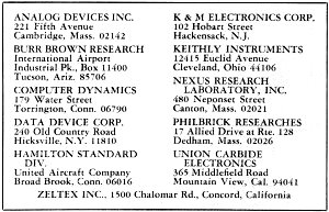
Table 2. Listing of modular-type operational-amp manufacturers.
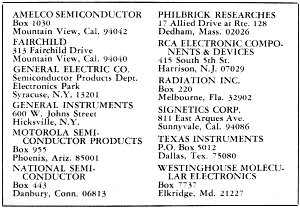
Table 3. Listing of integrated-circuit op-amp manufacturers. Industrial Op-Amp Applications Generally speaking, the modular units are being replaced in some cases by the integrateds, but at present, each package style offers some clear-cut advantages. Table 1 compares the two packages. The IC versions offer low cost, small size, and very low drift, while the modular versions offer higher input impedances, higher gain, and higher output power capability. Three low-cost readily available IC op amps appear in Figs. 2, 3, and 4. Here, their schematics and major performance characteristics are compared. Devices similar to these at even lower cost may soon be available. A directory of op amp makers is given in Tables 2 and 3. We can split the op-amp applications into roughly three categories: the industrial circuits, the computer circuits, and the active network synthesis circuits. The industrial circuits are "ordinary" ones, which will carryover into the consumer and commercial fields with little change. The boxed copy (facing page) sums up the mathematics. An operational amplifier is often used in conjunction with two passive networks, an input network, and a feedback network, both of which are normally connected to the inverting input. The gain of the over-all circuit at any frequency is given by the equation shown. It is simply the ratio of the feedback impedance to the input impedance at that frequency. For the circuits shown, a low impedance path to ground must exist for all input sources to allow a return path for base current in the two input transistors. Fig. 5A shows an inverting gain-of-100 amplifier useful from d.c. to several hundred kHz. The basic equation tells us the gain will be -10,000/100 = -100. The 100-ohm resistor on the "+" input provides base current for the "+" transistor and does not directly enter into the gain equation. It may be adjusted to obtain a desired drift or offset characteristic. The higher the gain of the op amp, the closer the circuit performance will be to the calculated performance. In the -of-100 amplifier, if the op amp gain is 1000, the gain error will be roughly 1 %. The exact value of the gain also depends upon the precision to which the input and feedback components are selected. Choosing different ratios of input and feedback impedances gives us different gains. Fig. 5B shows a gain-of-10 amplifier with a d.c. to 2 MHz frequency response and a 1000-ohm input impedance. We might ask at this point what we gain by using an op amp in this circuit instead of an ordinary single transistor circuit. There are several important answers. The first is that the input and output are both referenced to ground. Put in zero volts and you get out zero volts. Put in -400 millivolts and you get out +4 volts. Put in 400 millivolts you get out -4 volts. Secondly, the output impedance is very low and the gain will not change if you change the load the op amp is driving, as long as the loading is light compared to the op amp's output impedance. Finally, the gain is precisely 10, to the accuracy you can select the input and feedback resistors, independent of temperature and power-supply variations. It is this precision and ease of control that makes the operational amplifier configuration far superior to simpler circuitry. If the output is connected to the "-" input and an input directly drives the "+" input, the unity-gain voltage follower of Fig. 5C results. This configuration is useful for following precision voltage references or other voltage sources that may not be heavily loaded. The circuit is superior to an ordinary emitter-follower in that the offset is only a millivolt or so instead of the temperature-dependent 0.6-volt drop normally encountered, and the gain is truly unity and not dependent upon the alpha of the transistor used. By making the gain of the op amp frequency-dependent, various filter configurations are realized. For instance, Fig. 5D shows a band-stop amplifier. For very low and very high frequencies, the series RLC circuit in the feedback network will be a very high impedance and the gain will be -10,000/1000 = -10. At resonance, the series RLC impedance will be 100 ohms and the gain will be -100/1000 = -0.1. The gain drops by a factor of 100:1 or 40 decibels at the resonant frequency. The selection of the LC ratio will determine bandwidth, while the LC product will determine the resonant frequency.
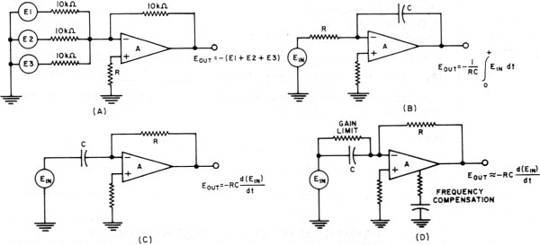
Fig. 5. Industrial op-amp circuits. (A) Gain-of-100 inverting amplifier. (B) Gain-of-10 inverting amplifier. (C) Unity-gain high input Z amplifier. (D) Band-stop amplifier. (E) Band-pass amplifier. (F) Precision ramp or linear saw-tooth generator. (G) Detector with low offset. (H) Logarithmic amplifier. (I) Voltage comparator. (J) Sine-wave oscillator. Fig. 5E does the opposite, producing a response peak at resonance 100 times higher than the response at very high or very low frequencies, owing to the very high impedance at resonance of a parallel LC circuit. More complex filter structures may be used to obtain any reasonable filter function or response curve. Audio equalization curves are readily realized using similar techniques. Turning to some different applications, Fig. SF shows a precision ramp generator. Operation is based upon the current source formed by the reference voltage and 1000-ohm resistor on the input. In any op-amp circuit, the current that is fed back to the input must equal the input current, for otherwise the"-" input will have a voltage on it, which would immediately be amplified, making the input and feedback currents equal. A constant current to a capacitor linearly charges that capacitor, producing a linear voltage ramp. The slope of the ramp will be determined by the current and the capacitance, while the linearity will be determined by the gain of the op amp. A sweep of 0.1-percent linearity is easily achieved. The output ramp is reset to zero by the switch and the 10-ohm current-limiting resistor. For synchronization, S may be replaced by a gating transistor. A negative input current produces a positive voltage ramp at the output. Note that the sweep linearity and amplitude is independent of the output loading as long as the load impedance is higher than the output impedance of the op amp. Ramps like this are often used in CRT sweep waveform generation, analog-to-digital converters, and similar circuitry. Silicon diodes normally have a 0.6-volt offset that makes them unattractive for detecting very low signal levels. If a diode is included in the feedback path of an operational amplifier, this offset may be reduced by the gain of the circuit, allowing low-level detection. Fig. 5G is typical. Here the gain to negative input signals is equal to unity, while the gain to positive input signals is equal to 100. The diode threshold will be reduced to 0.6 volt/100 = 6 millivolts. Another diode op-amp circuit is that of Fig. 5H. Here the logarithmic voltage-current relation present in a diode makes the feedback impedance decrease with increasing input signals, reducing the circuit gain as the input current increases. The net result is an output voltage that is proportional to the logarithm of the input, and the circuit is a logarithmic amplifier. This configuration only works on negative-going inputs and is useful in compressing signals measuring decibels, and in electronic multiplier circuits where the logarithms of two input signals are added together to perform multiplication. An operational amplifier is rarely run "wide open", but Fig. 51 is one exception. Here the op amp serves as a voltage comparator. If the voltage on the "-" input exceeds the "+" input voltage, the op amp output will swing as negative as the supply will let it, and vice versa. A difference of only a few millivolts between inputs will shift the output from one supply limit to the other. Feedback may be added to increase speed and produce a snap action. One input is often returned to a reference voltage, producing alarm or a limit detector. Op amps may also be used in groups. One example is the low-distortion sine-wave oscillator of Fig. 5J, in which three op amps generate a precision sine wave. Both sine an cosine outputs, differing in phase by 90° are produced. An external amplitude stabilization circuit is required, but not shown. Output frequency is determined solely by resistor and capacitor values and their stability. Computer Circuits The analog computer industry was the birthplace and once the only home of the operational amplifier. In fact the name comes from the use of op amps to perform mathematical operations. Many of these circuits are of industry-wide interest and use. Perhaps the simplest op-amp circuit is the inverter. This is an op amp with identical input and feedback resistors Whatever signal gets fed in, minus that signal appears the output, thus performing the sign-changing operation. Addition is performed by the circuit of Fig. 6A. Here the currents from inputs E1, E2, and E3 are summed and the negative of their sum appears at the output. Since the negative input is always very near ground because of feedback, there is no interaction among the three sources Resistor R is adjusted to obtain the desired drift performance. By shifting the resistor values around, the basic summing circuit may also perform scaling and weighting operations. For instance, a 30,000-ohm feedback resistor would produce an output equal to minus three times the sum of the inputs; a smaller feedback resistor would have the opposite effect. By changing only one input resistor without changing the other, one input may be weighted more heavily than the other. Thus, by a suitable choice of resistors, the basic summing circuit could perform such operations as EOUT= -0.5 (E1 + 3E2 + 0.6E3). Subtraction is performed by inverting one input signal and then adding. Two very important mathematical operations are integration and differentiation. Integration is simply finding the area under a curve, while differentiation involves finding the slope of a curve at a given point. The op-amp integration circuit is shown in Fig. 6B, while the differentiation circuit is shown in Fig. 6C. The integrator also serves as a low-pass filter, while the differentiator also serves as a high-pass filter, both with 6 dB/octave slopes.
Fig. 6. Computer operational-amplifier circuits. (A) Addition. (B) Integration. (C) Differentiation. (D) Practical operational-amplifier differentiator.
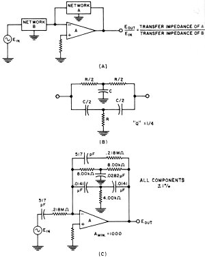
Fig. 7. Operational amplifiers in active network synthesis. (A) One form of active filter. (B) A twin-T network is identical to an LC parallel resonant circuit except for the "Q". (C) Circuit to realize "Q" of 14 without using an inductor. The differentiator circuit's gain increases indefinitely with frequency, which obviously brings about high-frequency noise problems. The circuit cannot be used as shown. Fig. 6D shows a practical form of differentiator in which a gain-limiting resistor and some high-frequency compensation have been added to limit the high-frequency noise, yet still provide a good approximation to the derivative of the lower frequency inputs. These two circuits are very important in solving advanced problems, particularly mathematics involving differential equations. Since most of the laws of physics, electronics, thermodynamics, aerodynamics, and chemical reactions can be expressed in differential-equation form, the use of operation amplifiers for equation solution can be a very valuable and powerful analysis tool. Active Network Synthesis Fig. 7. Operational amplifiers in active network synthesis. (A) One form of active filter. (B) A twin-T network is identical to an LC parallel resonant circuit except for the "Q". (C) Circuit to realize "Q" of 14 without using an inductor. Perhaps the newest area in which operational amplifiers are beginning to find wide use is in active network synthesis. There is increasing pressure in industry to minimize the use of inductors. Inductors are big, heavy, expensive, and never obtained without some external field, significant resistance, and distributed capacitance. Worst of all, no one has yet found any practical way to stuff them into an integrated-circuit package. If we can find some circuit that obeys all the electrical laws of inductance without the necessity of a big coil of wire and a core, we have accomplished our purpose. Operational amplifiers are extensively used for this purpose. One basic scheme is shown in Fig. 7 A. If two networks are connected around an op amp as shown, the gain will equal the ratio of the transfer impedances of the two networks. Since we are using three-terminal networks, and since the op amp is capable of adding energy to the circuit, we can do many things with this circuit that are impossible with two-terminal passive resistors and capacitors. Fig. 7B shows an interesting three-terminal network called a twin-T circuit. It exhibits resonance in the same manner as an ordinary LC circuit does. It has one limitation - its maximum "Q" is only 1/4. If we combine an op amp with a parallel twin- T network, we can multiply the "Q" electronically to any reasonable level. A gain of 40 would bring the "Q" up to 10. We then have a resonant "RLC" circuit of controllable center frequency and bandwidth with no large, bulky inductors required even for low-frequency operation. One example is shown in Fig. 7C where an operational amplifier is used to realize a resonant effect and a "Q" of 14 at a frequency of 1400 Hz. As the desired "Q" increases, the tolerances on the components and the gain become more and more severe. From a practical standpoint, value of "Q" greater than 25 are very difficult to realize at the present time. Note that the entire circuit shown can be placed in a space much smaller than that occupied by the single inductor it replaces.
Posted February 27, 2019 |
|||||||||||||
 |
|||||||||||||
|
|||||||||||||


|
||||||||||||||||||||||||||||||||||||