|
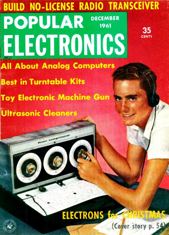
December 1961 Popular Electronics
 Table of Contents Table of Contents
Wax nostalgic about and learn from the history of early electronics. See articles
from
Popular Electronics,
published October 1954 - April 1985. All copyrights are hereby acknowledged.
|
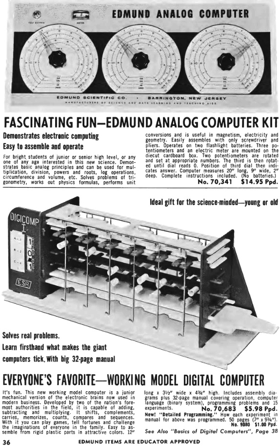
Edmond Analog Computer (Computarium LCD
website)
Analog computers are said to be the oldest form of computer, but I maintain digital
computers predated analog computers by millennia. That's right, our ancient forebears
certainly counted using their fingers and toes (aka digits) for addition and subtraction
long before anyone assembled a mechanism for performing mathematical operations.
Astronomers were some of the most prolific inventors of analog computers for determining
the positions of planets, moons, comets, and even longitude and latitude upon the
face of the Earth. Charles Babbage made one of the most famous mechanical computers
- the Babbage Difference
Engine. Probably the most widely used analog computer is one form or another
of a slide rule. I say one form or another because many of the
cardboard
type calculators are forms of slide rules. One type of analog computer we
use in the RF business everyday is a frequency mixer, which takes two numbers
(frequencies) and produces the sum and difference. This 1961 issue of Popular Electronics
magazine reports on a couple low cost analog computers available at the time, including
the three-dial Edmonds Analog Computer that appeared in advertisement in many technical
magazines of the day.
An Introduction to Analog Computers
 Now you can take your first step into the
fascinating world of electronic brains Now you can take your first step into the
fascinating world of electronic brains
By Julian M. Sienkiewicz, Managing Editor
For centuries man has been utilizing simple analog devices to solve mathematical
problems by analogy. In other words, numbers are converted into something else which
can be worked with more easily than the numbers themselves. One everyday example
is the slide rule, which converts numbers into distances, then reconverts the summed
distances into numbers, providing a solution. Anyone who has multiplied two numbers
on a slide rule will testify to its operating ease, rapid solution, and remarkable
accuracy.
This article will go one step beyond the slide rule and describe a direct-reading
analog computer which will solve simple addition and multiplication problems, extract
roots, and perform trigonometric operations. So simple is this computer that it
could be called an "electronic slide rule."
Voltage Analog. An ordinary potentiometer will help us see how
a number can be converted into a voltage analog. Figure 1 shows a simple circuit
of a potentiometer, R1, connected in series with a battery, B1. Rotating the dial
pointer on the shaft of R1 causes the potentiometer wiper to "pick off" a voltage
proportional to the dial setting.
In Fig. 1, the dial is calibrated from zero to one and the voltage supplied by
the battery is 1.0 volt. Thus, in this particular instance, the dial setting indicates
the voltage at the wiper of the potentiometer. A voltmeter connected at the output
terminals of this circuit will indicate the setting of the dial -0.36 volt
would mean that the dial is set at 0.36 unit. The voltage is an analog voltage,
since it may represent a dial quantity of 0.36 acre, quart, or even light year.
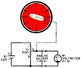
Fig. 1 - A potentiometer can be used to convert dial settings
to correspondingly equal voltages. When the dial is set at 0.36, the wiper picks
off 0.36 volt d.c.
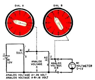
Fig. 2 - Two cascaded potentiometers develop voltage analog equal
to product of the dial settings.
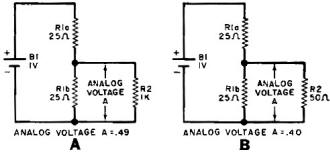
Fig. 3 - Circuits showing cause for loading error (A) when R2
is 1000 ohms, (B) when R2 is 50 ohms.
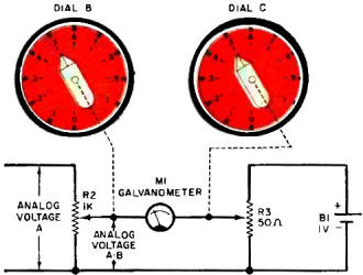
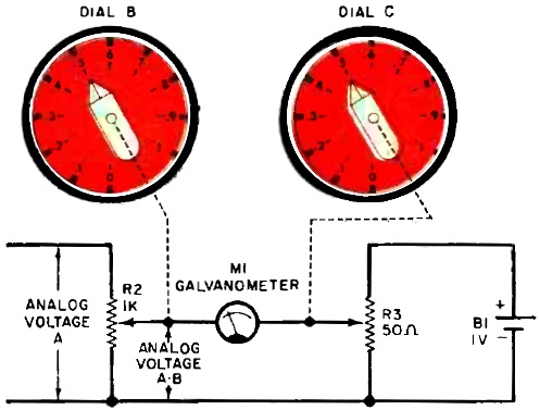
Fig. 4 - No loading error occurs when voltage on wiper of R3
equals analog voltage AB, or 0.5 volt.
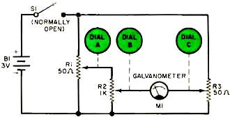
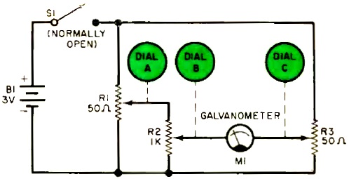
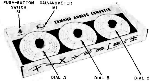
Fig. 5 - Schematic diagram of a three-potentiometer analog computer
with a galvanometer (M1) null indicator. Switch S1 is depressed in order to read
M1.
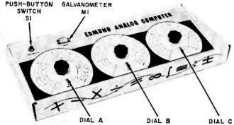
Fig. 6 - Circuit components seen on front panel of Edmund Analog
Computer are identified here. Each dial has four concentric scales.
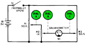
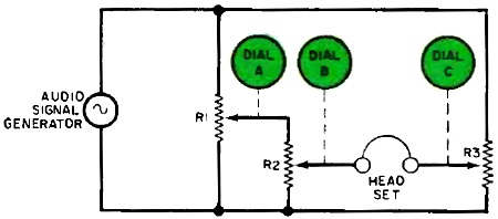
Fig. 7 - Simplified schematic of G.E.'s "Project 4" computer.
Headset is used to detect sound nulls.
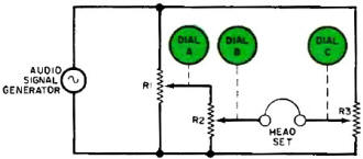
Fig. 8 - Dials on Edmund Analog Computer have four scales each,
while G.E.'s kit has more but unclutters scales by using removable dial scale plates.
Multiplying. In Fig. 1, a voltage analog for the number 0.36
was developed at the wiper of R1. It can also be said that the supply voltage across
R1 was multiplied by 0.36. Thus, 1.0 volt times 0.36 will be 0.36 volt. If a voltage
other than 1.0 volt were supplied by B1 in Fig. 1, we would be multiplying the supply
voltage by the dial setting.
This apparent ability of potentiometers to multiply can best be seen in Fig.
2. Battery B1 supplies 1.0 volt across potentiometer R1. Dial A is set at 0.36 so
that analog voltage A developed at the wiper of R1 (0.36 volt) is applied across
potentiometer R2. Dial B is set at 0.50 so that the voltage at the wiper of R2 will
be only 0.50 times the voltage across R2, or simply 0.36 x 0.50. The voltage developed
at the wiper of R2 is appropriately called analog voltage A-B, and voltmeter M1
will indicate this voltage to be 0.18 - the product of 0.36 and 0.50.
Loading Error. Looking again at Fig. 2, you will note that the
value of potentiometer R1 is 50 ohms, whereas potentiometer R2 is a 1000-ohm unit.
The reason for this is quite simple, provided you down-gear your thinking from analog
computers to simple d.c. networks. Figure 3(A) corresponds to Fig. 2 when the wiper
of R1 is set at 0.50 or mid-position. Hence, R1a in Fig. 3(A) represents the "top
half" of R1 in Fig. 2 (the portion between terminals 1 and 2). Likewise, R1b represents
the "bottom half" of R1 (the portion between terminals 2 and 3). We know from the
dial setting that analog voltage A should be 0.50 volt. However, let's see what
analog voltage A actually is in Fig. 3(A).
First, since R1b and R2 are in parallel, their combined resistance is approximately
24.4 ohms. Using Ohm's law, we find that the voltage drop across R1b (in parallel
with R2) is approximately 0.49 volt. This means that R2 in Fig. 2 will tend to lower
the true value of analog voltage A and introduce a small error. In the case cited,
the error is only 2% - not much for this simple computer circuit.
In Fig. 3(B) , the value of R2 was selected as 50 ohms solely to illustrate the
loading effect of R2 on R1b. In this instance, the combined resistance of R1b and
R2 is approximately 17 ohms. Again resorting to Ohm's law, we find analog voltage
A developed across R1b and R2 to be approximately 0.40 volt. Compared to the desired
analog voltage of 0.50, the loading effect of a 50-ohm potentiometer will introduce
an error of 20% - an excessive amount for most purposes.
It should be evident, then, that when two potentiometers are connected as shown
in Fig. 2, the second one (R2) should be many times larger than the first one (R1).
However, do not be tempted into believing a potentiometer with a very large resistance
- one megohm, say - will completely solve our loading problem. Even if the resistance
value of the second potentiometer is very large, a voltmeter connected across its
wiper and bottom terminal will also cause a loading effect and hence introduce error.
This is due to the resistance of the voltmeter itself - usually only several thousand
ohms.
Galvanometer Indicator. One method of removing the loading effect
of the voltmeter (M1) used in Fig. 2 is to replace it with an indicator that requires
no current to indicate the analog voltage developed by a potentiometer. Such a device
is the galvanometer indicator shown schematically in Fig. 4.
Close inspection of the circuit in Fig. 4 reveals that current will flow though
galvanometer M1 whenever the wipers of potentiometers R2 and R3 select voltages
that are not equal. This condition causes the galvanometer pointer to deflect either
to the left or right of its normal "center rest" or "zero deflection" position.
Since dial B is preset to "some number" input, as described earlier, it remains
for dial C to be adjusted until the voltage at the wiper of R3 equals the voltage
at the wiper of R2. When this occurs, the voltage drop across the galvanometer is
zero, resulting in zero current through the galvanometer and no deflection of the
meter's pointer. Dial C, which is calibrated to convert the voltage picked off by
R3 to numbers, indicates the correct value of analog voltage A.B. Since the electrical
components M1 and R3 draw no current from R2, there is no loading on the analog
circuits and no errors are introduced into the electrical computations by the galvanometer.
An important fact to note in Fig. 4 is that potentiometer R3 has a value of 50
ohms. This is permissible, since (1) R3 does not load the computer circuits when
the correct answer is set on dial C and (2 ) the lower value is desired so that
when an incorrect answer is selected the deflection of M1 will be large due to the
large currents flowing through the galvanometer movement. This large deflection
due to an incorrect answer enables the computer operator to adjust dial C accurately
for a galvanometer null or zero deflection. In operation, of course, the galvanometer
deflects either to the right or left of its center position, depending upon whether
the wiper of R3 is positive or negative with respect to the wiper of R2.
Complete Circuit. The simple analog computer circuit shown in
Fig. 5 is identical to the one used in the analog computer kit made by the Edmund
Scientific Co., Barrington, N. J. (see Fig. 6 ) and is the culmination of the circuits
shown in Figs. 1 through 4.
Two interesting points should be noted: the first one is that the battery voltage
of B1 is 3 volts. Previously in our discussion, we used a "1-volt" battery for B1.
This variance in voltage suggests that the voltage of B1 is not critical, as is
actually the case.
Examine Fig. 5 carefully and note that B1 is connected across two resistive legs:
the summed resistances of R1 and R2, and the resistance of R3. Galvanometer M1 is
used to detect a zero voltage difference between the resistive legs exactly like
its counterpart in the Wheatstone bridge. Therefore, as long as the two resistive
legs receive the same voltage, its value is unimportant.
The second point to be noted in Fig. 5 is that a switch (S1) has been added.
This push-button switch is nothing more than an on/off switch for reducing battery
drain. It is depressed only after dials A and B have been set to desired values
and dial C is being adjusted so that the galvanometer indicates a null.
Sound Null. Another good way to determine when the analog computer
is tuned to a null (correct answer), is to listen for it rather than look for it.
In the Edmund computer, a null can be seen when the galvanometer is not deflected.
In an analog computer kit made by General Electric (see cover photo),the galvanometer
has been replaced with a headset; since the headset can only detect audio signals,
the computer potentiometers are powered by an audio signal generator and not by
dry cells. Except for these two changes, the General Electric analog computer kit
is electrically identical to the Edmund kit.
Figure 7 is a simplified schematic drawing of the G.E. analog computer circuit.
To operate, the computer potentiometers are preset to fixed input quantities and
the "answer" potentiometer (connected to the C dial) is rotated until the audio
sound is no longer heard in the headset.
[borders/_temp/2-28-2024/google-300x250-ad-unit-included-file-left.htm]Dials. The dials for both the Edmund and General Electric kits
are accurately calibrated so that many complex problems can be performed. The similarity
of the dials found in each kit can be seen in Fig. 8.
The Edmund dials include a linear scale plus logarithmic and trigonometric scales,
whereas the General Electric dials have in addition "squared" and reciprocal scales.
Instruction manuals provided with both kits give detailed instructions on how to
use these dials to solve many typical problems closely related to electrical technology
and science.
A Fraction of the Field. The "ground floor" introduction to
analog computers which you have just read naturally covers but a very small fraction
of the total analog computer field. Besides potentiometers, meters, and switches,
manufacturers of analog computers also use synchros, two and three-dimensional cams,
linkages, gears, and complex electronic circuits to perform the countless specialized
functions the human mind may require of a machine.
If you find the subject of analog computers interesting and this ground floor
introduction just whets your appetite, you might want to visit your public or school
library. Each day, more and more books on this timely subject are being placed on
library shelves. Look for them, and be kind to that gent who beat you there - he
may be the author of this article!
Posted September 1, 2023
|