|
August 1972 Popular Electronics
 Table of Contents Table of Contents
Wax nostalgic about and learn from the history of early electronics. See articles
from
Popular Electronics,
published October 1954 - April 1985. All copyrights are hereby acknowledged.
|
A lot of us still use
older test equipment at home and even in the company lab. As discussed in this 1972
article from Popular Electronics magazine, the displayed rise time on an
oscilloscope display is not necessarily that true rise time of a signal - particularly
when the speed approaches the rated bandwidth of the equipment. In that case, it
is necessary to mathematically compensate for the rise times of each individual
component used for making the measurement. Hooking the o-scope probe tip to the
calibration point on the front of the instrument and adjusting the probe's trim
capacitor for a flat response is not always good enough. Most modern o-scopes can
calculate and apply corrections automatically, negating the need for a manual correction.
If your application is not super critical from a timing standpoint, then you do
not need to bother with correction, but it is worth keeping rise time measurement
inaccuracies in mind just in case you run into an otherwise inexplicable problem
that may turn out to be a timing issue.
Rise-Time Measurements - What You See My Not be What You've Really Got
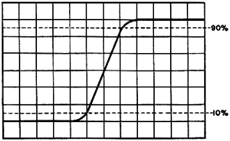
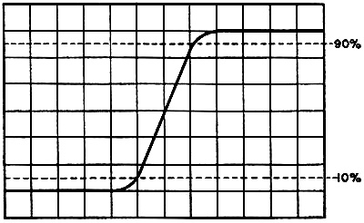
Fig. 1 - Pulse rise time is measured between the 10% and
90% points on the leading edge of oscilloscope trace. In this case, rise time is
100 nanoseconds.
By Raymond E. Herzog
Suppose you feed the output of a pulse generator through a probe to an oscilloscope.
You adjust the scope time base for a fast sweep. (This is the typical setup for
measurement of rise time.) The result is the easily recognized rise-time waveform
shown in Fig. 1.
Question
If the time base is set for a sweep of 50 nanoseconds
per division, what is the rise time of the generator's output pulse - ignoring any
inherent scope inaccuracies.
"That's easy," you say, quickly multiplying 50 ns/div times the two divisions
covered by the pulse's leading edge. "100 ns is the rise time of the pulse. Right?"
Maybe yes; and maybe no!
Although 100 ns is the correct reading of the scope display, this value may not
be the true rise time of the pulse. So ignoring scope inaccuracies, what other reason
is there for suspecting that the measurement is not the real rise time?
Basically it is that, when the pulse passes through the probe, the scope amplifier,
and even the scope CRT, it suffers rise time deterioration. Thus, the displayed
waveform can't represent the true, original signal.
Although this is an unfortunate circumstance, it has one saving grace: it can
be predicted. So, if you erroneously said that the rise time in the example was
100 ns, it should be both interesting and informative to learn how to determine
what the error might be.
Rise-Time Formula
True rise time can be determined by the use
of the tongue-twisting formula known as "the square root of the sum of the squares."
In mathematical terms:

where TRG = true signal generator rise time
TRD = displayed rise time
TRP = probe rise time
TRO = oscilloscope (amplifier and CRT) rise time
For a low- to medium-priced general-purpose oscilloscope, a typical rise time
is 35 ns.
For a standard probe, rise time is 5 or 10 ns. Putting these values into the
formula, we get

Thus, the actual rise time of the generator pulse is 93.1 ns and not the 100
ns displayed on the scope; and the measurement was in error by 7.4%.
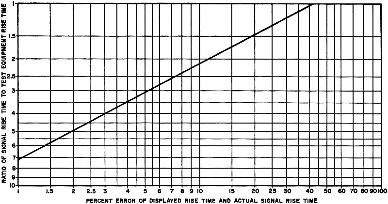
It is important, therefore, to keep in mind that the displayed rise time is greater
than the actual rise time. The amount of error is shown in Fig. 2, where per
cent of error is plotted against the ratio of the input signal's rise time to test
equipment rise time. In our example, this rise time ratio would be 93.1 divided
by the square root of 352 + 102 or 2.56.
Knowing that the measurement devices do introduce an error and with the aid of
Fig. 2, you can determine just what error to expect. Conversely, to make a
measurement within a given accuracy, Fig. 2 can be used to find what rise time
response is needed in the test equipment.

Fig. 2 - Measurement error is inversely proportional to
the rise-time ratio.
More About Rise Time
We often concern ourselves with only the
frequency response of an oscilloscope or an amplifier when, as we have seen, rise
time is also important.
In using Fig. 1, we measured rise time between the 10% and 90% points of
peak value on the leading edge of the pulse. These two points are used as standards
for waveform measurement in the industry.
Looking at Fig. 1 again, you will note that the pulse rises linearly from
the 10% voltage level to the 90% level. Such a characteristic is known as a Gaussian
response. When an ideal unit step pulse (one with zero rise time) is applied to
an amplifier (or cascaded amplifiers) whose frequency response is RC limited, the
response is Gaussian. For a Gaussian response, there is a relationship between rise
time and frequency (also called bandwidth):
0.35 = tr X bw
where tr = rise time in microseconds
bw = frequency bandwidth in MHz
Oscilloscope vertical amplifiers consist of cascaded RC stages so the above formula
applies. For instance, if a scope has a 10-MHz bandwidth, its corresponding rise
time would be 0.035 microseconds or 35 ns.
The 0.35 constant in the formula results from a combination of two factors:
RC rise time = tr = 2.2RC
-3 dB frequency = FC = 1/ (2πRC) Consider
first the 2.2RC factor and look at the universal time constant curve in Fig. 3.
This curve will readily be recognized as the capacitor charging voltage in a series
RC network with an applied ideal step pulse. Recalling that, in rise time measurements,
the 10% and 90% points were used, we find the corresponding RC value for these two
points: namely 0.1 RC and 2.3 RC. Taking the difference between these two values,
we get 2.2RC - the time in which rise time is resolved.
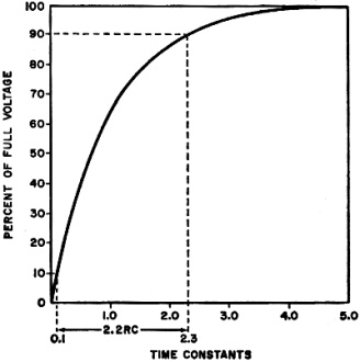
Fig. 3 - This is time constant curve for charging capacitor
in series RC circuit.
But Wait Just a Moment!
The curve in Fig. 3 is not Gaussian,
so how can it be used in our calculations? Well, irrespective of Gaussian - or whatever
- the universal time constant curve serves only as a reference for the 2.2 RC value.
It is not the signal pulse to be measured (as in Fig. 1) and thus does not
have to be Gaussian.
Remember that what we did say about Gaussian response was that it pertained to
an amplifier stage whose frequency response is RC limited.
This brings us to the second factor in the 0.35 constant: the -3-dB frequency,
or the frequency at which an amplifier's gain is down 3 dB from mid-frequency gain.
The influence of the stage's resistance and capacitance is shown in the -3-dB frequency
formula: FC = 1/ (2πRC).
Having defined these two factors, let's see how they determine the 0.35 constant.
First, transpose FC = 1/(2πRC) into RC
= 1/(2πFC).
Then from tr = 2.2RC, we get tr = 2.2. [1/(2πFC)]
= 0.35/FC. Finally, 0.35 = tr X FC. Or since frequency
response is bandwidth, 0.35 = v X bw.
Posted July 11, 2023
(updated from original post on 7/18/2017)
|