|
April 1953 QST
 Table of Contents Table of Contents
Wax nostalgic about and learn from the history of early electronics. See articles
from
QST, published December 1915 - present (visit ARRL
for info). All copyrights hereby acknowledged.
|
Here is a fairly major treatise on folded
and loaded antennas that appeared in a 1953 issue of QST magazine, with
"Suggestions for Mobile and Restricted-Space Radiators." It is not for the faint
of heart or anyone with math phobia or math anxiety. Integral calculus is part of the presentation,
although an understanding of calculus is not required to get the gist of the article.
Equations for calculating the antenna configuration radiation resistances are given
for the 3λ/4-wave folded dipole, the λ/8-wave folded monopole, the bottom-,
center- and top-loaded λ/8-wave monopole, the bottom-loaded λ/16-wave monopole,
and the λ/4-wave monopole folded twice, to name a few.
Folded and Loaded Antennas
Suggestions for Mobile and Restricted-Space Radiators
By William B. Wrigley,* W4UCW
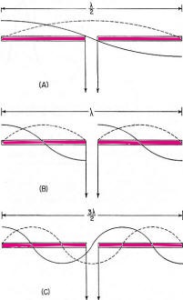
Fig. 1 - Current and voltage distribution on half-, one-,
and one and one-half wavelength antennas, fed at the center.
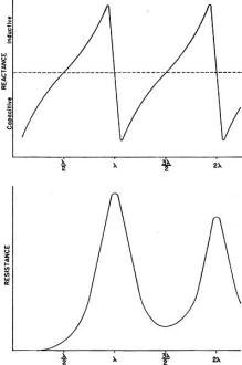
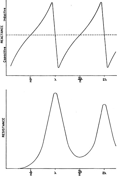
Fig. 2 - Variation of reactance and resistance at input
terminals of center-fed antennas as the total length is varied.
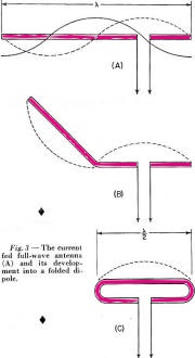
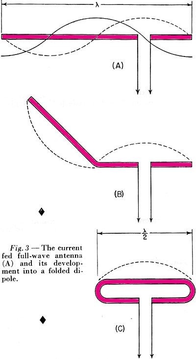
Fig. 3 - The current fed full-wave antenna (A) and its development
into a folded dipole.
Using a simplified method of calculation, the author develops values for the
radiation resistance of various folded and loaded forms of short antennas. Several
interesting possibilities for small radiating systems are discussed.
While we are all quite familiar with the half-wave folded dipole, its radiation
pat-tern, input or radiation impedance, and application to amateur installations,
it seems that there are many more folded configurations which are not well known
and which may prove quite surprising in their usefulness. Most of us are also reasonably
familiar with the basic methods of loading mobile antennas, but we may be surprised
at what a few simple calculations can tell us about the effects of various methods
of loading.
First let us consider the basic half-wave thin dipole1 with a theoretical
balanced center-feed impedance of about 72 ohms. Fig. 1A shows such an antenna
with its current distribution (dashed line) and charge distribution (solid line).
While these distributions are not exactly sinusoidal as shown, the assumption that
they are so introduces negligible error in impedance and field-pattern calculations,
and at the same time reduces these calculations from formidable complexity to fairly
simple operations. Now Fig. 1B shows what happens if we attempt to operate
this antenna at the second harmonic. We now have a condition of antiresonance. The
input resistance is much higher and the reactance variation with frequency is much
greater than in the original resonant case at the fundamental frequency. Fig. 10
shows the current distribution at the third harmonic, where we once again have a
reasonably broad resonant condition. Fig. 2 shows qualitatively this same information
as resistance and reactance plotted against antenna length in wavelengths.
We might conclude from all this that, at least in the symmetrical case, an antenna
will be rea-sonably broad-band only at frequencies where the length is an odd number
of half-wavelengths or such that the feed point is at a current maximum.
Why can we not simply move the feed point to a current maximum in the second-harmonic
case of Fig. 1B? We can, in fact, but then things change somewhat since the
now-continuous center cannot support a discontinuity in charge. So we get distributions
as shown in Fig. 3A, somewhat unbalanced, as would be expected. Since the
charge polarity is now the same at both ends, however, we can fold the left current
loop over the driven loop as shown in Fig. 3B and obtain the familiar folded
dipole of Fig. 3C, which is, of course, quite symmetrical. The impedance of
this folded arrangement can be found by considering it as merely an impedance transformer
between the feeder line and free space. The far-field intensity normal to the axis
of the antenna is proportional to the total current added up along both wires and,
since we now have exactly double the current producing the far field, as compared
to that in either wire alone (in particular the one being fed), we must have double
the far-field pattern strength. However, the transmission line furnishes power that
is exactly the same as in a simple dipole, hence the input or radiation resistance
must be directly proportional to the square of the total far-field intensity as
compared to that of the fed wire only (W = E2 / R). In this case 22
= 4 and 4 x 72 is 288 ohms, which is the approximate theoretical radiation resistance
of a thin folded half-wave dipole. It is well known that the reactance-frequency
variation of the antenna is, in this particular case, partially cancelled out by
the opposite variation of the two transmission line stubs in series seen from the
feed point such that the folded dipole has, in fact, broader bandwidth than the
single thin dipole.
Other Folded and Loaded Systems
Since this folding operation has proved so attractive, let us now investigate
the possibility of folding the configuration of Fig. 1A. Because of the mobile
antenna application we shall consider half the antenna of Fig. 1A against a
ground plane and fed with a coaxial cable as shown in Fig. 4A. We can fold
the antenna as in Fig. 4B and obtain the eighth-wave folded monopole of Fig. 4C?
Since the opposite ends of the original dipole were at opposite charge polarity
(Fig. 1A), we must leave these ends unconnected upon folding; or, in the ground
plane case, the folded-over section must not be allowed to contact the ground plane.
For radiation purposes, the current in the folded section is opposite in direction
to that of the unfolded half and one must be subtracted from the other, resulting
in the radiation current distribution shown in Fig. 4D.
Now in the folded dipole case we found the impedance by adding (mathematically
integrating) the current distribution along the wire to obtain a figure proportional
to far-field strength.
Actually, these figures of proportionality are only valid comparisons of two
antennas if the far-field patterns or current distributions are identical. However,
in all the cases we shall consider here, there will be only one combined radiating
current loop and hence only one far-field pattern lobe. These lobes will not be
exactly the same shape, but to assume them so is a reasonable approximation as evidenced
by the fact that the far-field radiation pattern of a half-wave dipole with sinusoidal
current distribution is only slightly more directive (78 degrees between half-power
points) than that of a minutely short dipole with uniform current distribution (90
degrees between half-power points).
As shown by the calculations in the Appendix, the approximate radiation impedance
of the folded eighth-wave monopole of Fig. 4D is 6.2 ohms. A similar analysis
of a bottom-loaded eighth-wave monopole, Fig. 4E, shows that its radiation
resistance also is 6.2 ohms, which is the same as for the folded case! This identity
holds for a quarter-wave monopole which is folded into any even number of elements
as compared to a bottom-loaded single element of the same actual height.
Fig. 4F shows the current distribution of a top-loaded eighth-wave monopole.3
The approximate radiation resistance, as shown in the Appendix, is 18 ohms. For
the center-loaded eighth-wave monopole of Fig. 4G the approximate method of
calculation still applies and leads to a theoretical radiation resistance of 11.5
ohms.
Folded Mobiles
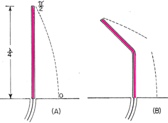
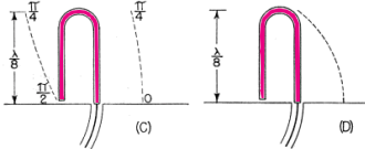
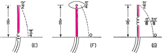
Fig. 4- Coaxial-fed quarter wave antenna and ground plane
(A); effect of folding (B, C and D); bottom-loaded eighth-wave (E), top-loaded eighth-wave
(F), and center-loaded eighth wave (G).
Fig. 4D could be interpreted as a 20-meter mobile antenna made up of two
adjacent eight-foot whips. One significant advantage of this arrangement is that
there is no loading-coil loss to contend with. A further advantage is in the realization
that a shorted stub of appropriate length (λ/4 at 20 meters) connected to
the mounting point of the folded or second whip will be an open circuit at 20 meters
and a closed circuit at 10 meters. At 10 meters the system becomes a quarter-wave
folded monopole (half a folded dipole) with an input impedance of a little over
100 ohms, while at 20 meters, with no mechanical change, it becomes an eighth-wave
folded monopole with an impedance of about 5 ohms. (Five ohms is probably closer
than the theoretical 6.2 ohms since mobile quarter-wave whips look more like 30
than 36 ohms. They are not "thin.") The rather severe difference in impedance between
the fundamental and second-harmonic case can be taken care of by feeding the pair
of whips with another quarter-wavelength of cable at 20 meters. Being a half-wave
at 10 meters, this would give a load impedance at the transmitter of somewhat over
100 ohms at 10 meters and Zo2 / 5 ohms at 20 meters, where
Zo is the characteristic impedance of the cable used. This double whip
10-20 system will be slightly more selective, however, than either of the plain
folded monopoles, since the reactance deviation with frequency of the shorted stub
is opposite in sign from that required to counteract the reactance deviation of
the antenna.
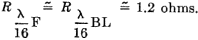
If a 40-meter quarter-wave monopole were folded down to eight-foot height there
would be four sections. The resulting impedance, which again is the same as that
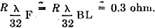
of a bottom-loaded sixteenth-wave monopole, is 1.2 ohms (see Appendix). An 80-meter
arrangement would take eight whips and would have an impedance of approximately
0.3 ohm. However, these latter two extensions of the folding process do not immediately
appear very attractive. To complete our discussion of folded and loaded monopoles
we should include the radiation resistances of 40- and 80-meter loaded antennas.
Table I shows all of these figures calculated by the far-field factor method and
based on a nominal quarter-wave monopole impedance of 30 ohms, more realistic than
the theoretical "thin" monopole value of 36 ohms.
It is interesting to investigate the impedances of short monopoles with optimum
current distributions. This requires loading at both top and bottom so as to center
the current loop on the antenna as shown in Fig. 5. The values of radiation
resistance for 40 and 80 meters are also included in Table I.
A top- and bottom-loaded (current loop centered) 10-meter quarter-wave monopole
has the very attractive impedance of 120 ohms, calculated by this method. The ground
current losses in it would be considerably less than the losses in the unloaded
case for the same radiated power.
Comparisons
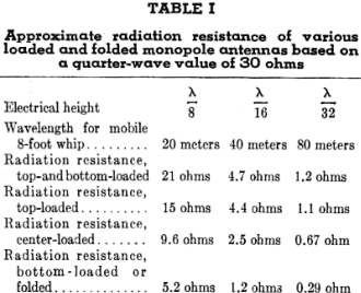
Table I - Approximate radiation resistance of various loaded
and folded monopole antennas based on a quarter-wave value of 30 ohms
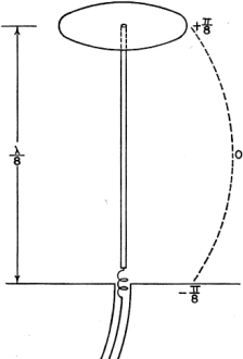
Fig. 5 - Top- and bottom-loaded eighth-wave coax-fed antenna
with ground plane.
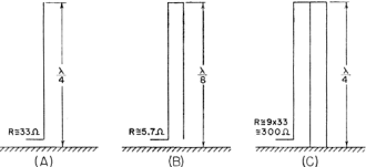
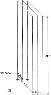
Fig. 6 - Quarter-wave antenna with ground plane (A); same
folded to height of one-eighth wave (B); three-wire folded quarter-wave monopole
and ground plane (C); same folded to one-eighth-wave height, with dimensions for
1.85 Mc. (D). The approximate radiation resistance for the last case is 9 X 5.7
= 51 ohms.
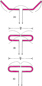
Fig. 7 - Center-fed antenna one and one-half wavelength
long (A) folded into a three-quarter-wave folded dipole (B and C).
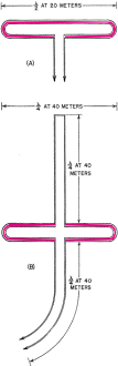
Fig. 8 - An antenna system for 7, 14 and 21 Mc., using a
shorted stub to act as an automatic switch for various bands.
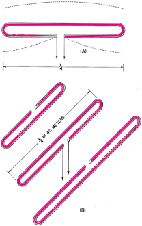
Fig. 9 - A possible 40-meter beam arrangement using quarter-wave
folded elements.
We can now draw some very definite conclusions regarding the merits of various
loading schemes. Since the principal loss in a vertical radiator (outside of the
loading-coil loss) is due to ground currents, the efficiency rapidly decreases with
decreasing radiation resistance. For constant radiated power, the current must be
greater for smaller values of radiation resistance. Greater current means greater
loss and consequent reduction in efficiency; therefore, the power loss in a center-loaded
eighth-wave monopole is more than that of a top-loaded equivalent antenna and the
loss in the bottom-loaded case is more than that of the center-loaded case. A combination
of both top and bottom loading, however, gives a radiation impedance which in some
cases reduces the loss to an exceptionally low value compared to that of the bottom-only
loaded, folded, or unloaded case. Sufficient top loading is usually impractical,
however, particularly in the case of very short monopoles.
The main conclusion we can draw from all these calculations is that short antennas
(monopoles less than one-tenth wavelength) have uncomfortably low radiation resistances
and practically nothing can be done to improve their efficiencies to a reasonable
value, except possibly by using a multiwire system to raise the impedance as described
earlier. On the other hand, the efficiencies of longer (quarter- or eighth-wave)
monopoles may be increased considerably by proper loading, or folding. A practical
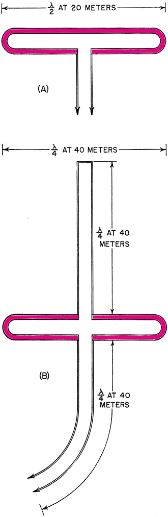
example is the 160-meter folded eighth-wavelength three-wire monopole shown in Fig. 6B.
Adding a third wire to the folded quarter-wave monopole, Fig. 6C, raises the
resistance to about 300 ohms, and when this antenna is folded over as shown in Fig. 6D,
the radiation resistance becomes about 50 ohms, a good match for coaxial cable.
Suggested dimensions for 1850 kc. are given in the sketch.
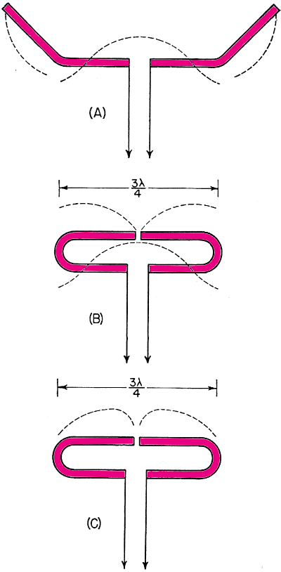
3λ/4 Folded Dipole
Now, since we have pretty well folded and loaded Fig. 1A, let us investigate
the results of folding Fig. 1C. This process and the resulting current distribution
is shown in Fig. 7 where the center line represents a ground plane for the
vertical analogue of the system. Calculation leads to an impedance for this three-quarter
wave folded dipole of about 420 ohms. J. D. Kraus 5, 6 (W8JK) has measured
one of these to be about 450 ohms. The new 21-Mc. band makes this arrangement quite
useful as can be seen in the following scheme:
Suppose we start with the 20-meter folded dipole of Fig. 8A and open-circuit
the top dipole opposite the feed point. We now have a quarter-wave folded dipole
at 40 meters, the vertical analogue of which we have already discussed. The impedance
of this dipole at 40 meters should be about 12 ohms. A λ/4 length of Twin-Lead
at 40 meters would then transform this to Zo2/12 at the transmitter.
A shorted λ/4 stub connected to the open ends of the dipole as shown in Fig. 8B
would provide an open circuit at 40 meters, a short circuit (λ/2) at 20 meters,
and open again (3λ/4) at 15 meters. At 20 meters we have our original half-wave
folded dipole and at 15 meters we have our 3λ/4 folded dipole. In this last
case the now 3λ/4 feed line transforms the impedance to Zo2/420
at the transmitter. Of course, the shorted stub may be folded up in some convenient
way so as not to consume all the space indicated in Fig.8B.
The radiation patterns of the antenna are practically identical at all three
frequencies.
Other Possibilities
No doubt there are many more folded arrangements which may prove attractive,
such as the possibility of a 40-meter close-spaced beam made up of quarter-wave
folded dipoles. Now, due to the coupling of the parasitic elements, the impedance
of the driven element would be considerably lower than the 10 to 12 ohms of a folded
quarter-wave dipole in free space. This may be raised to a more reasonable value,
however, by feeding at the current node (voltage feed) rather than at the current
loop.2 The driven element would then look just like a 20-meter folded
half-wave dipole, but the current distribution would be as shown in Fig. 9A
and the entire array would look something like Fig. 9B. A T-match or a "Q"-section
at the feed point may provide an even better driving-point impedance. The approximate
over-all lengths of the elements, before folding, may be determined from the curves
for 20-meter elements given in The Radio Amateur's Handbook or in the ARRL Antenna
Book, simply by dividing the frequency scale in half and doubling the length scale.
With some compromise in element spacing this array may even be operated as a
combination 40-20-15 beam by the use of small lumped networks in the parasitic elements
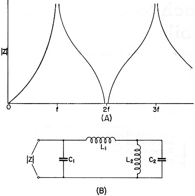
in place of the rotationally cumbersome stubs of Fig. 8B. In case you would
like to try this latter arrangement, Fig. 10A shows the impedance vs. frequency
characteristic required and Fig. 10B shows a suitable network to accomplish
this. The parameter K allows for variation in the over-all impedance level, but
should be chosen so as to make C1 a conveniently small capacitor and
include the capacity between the two ends of the element. Since harmonic antennas
are not, in general, exact multiples of length, all the network elements may require
some adjustment after final assembly to approach resonance on all three bands.
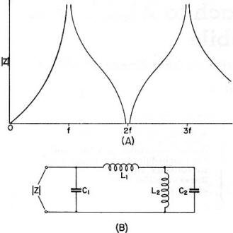
Fig. 10 - Impedance variations in the frequency range of
interest (A) and a lumped-circuit equivalent of the stub shown in Fig. 8. Component
values can be calculated from the following formulas, where f is in megacycles:
C1 = K μμfd.
C2 = 2.4K μμfd.
L1 4220/Kf2 μh.
L2 = 1.67 L1 μh.
The factor K may be chosen to make the inductances and capacitances come out
to convenient or constructionally-feasible values.
Appendix A
λ/8 Folded Monopole Antenna Radiation Resistance (Fig. 4C)
To find the radiation impedance of the eighth-wave folded monopole we must find
the far-field figure of proportionality normal to the axis of the antenna by subtracting
the integrated current of the folded-over half from the integrated current of the
unfolded half. The total length is
λ/4 or π/4
radians so
= 0.707 - 0 - 1.00 +0.707 = 0.414.
This is the far-field proportionality constant whose square must be compared
with that of a known antenna to give the impedance. The known standard is, of course,
the thin quarter-wave monopole whose figure is
and whose theoretical input impedance is about 36 ohms.
Therefore, the approximate radiation impedance of the thin folded eighth-wave
monopole is
Bottom-Loaded λ/8 Monopole Antenna Radiation Resistance (Fig. 4E)
The current distribution on a bottom-loaded eighth-wave monopole, Fig. 4E,
is identical with the top half of the quarter-wave monopole which we folded over
in the previous case, since the loading coil merely replaces the missing half. We
can calculate the radiation resistance of the remaining half as follows:
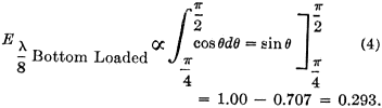
1.00 - 0.707 = 0.293.
This far-field figure, however, concerns the impedance referred to a current
maximum point and since we are feeding at the
π/4 or 45-degree
point we must divide by the square of the cosine of 45 degrees (constant power impedance
is inversely proportional to the square of the current). So finally we get
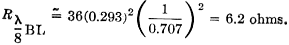
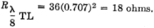
Top-Loaded λ/8 Monopole Antenna Radiation Resistance (Fig. 4F)
The approximate radiation resistance can be calculated from the cosine integral
from 0 to π/4 which gives a far-field factor of 0.707.
Center-Loaded λ/8 Monopole Antenna Radiation Resistance (Fig. 4G)
For the center-loaded case the calculation is a little more complicated. but
our approximate method still applies. The far-field factor includes two additive
components, the first of which comes from the bottom section of the antenna and
is merely the cosine integral from 0 to
π/8. The
loading coil effectively replaces the missing center half of the antenna so that
the current distribution along the top section is essentially the cosine curve from
3π/8 to
π/2. Since
the current is continuous through the coil, however, this second integral must be
multiplied by the ratio of the cosines of
π/8 and
3π/8. The
approximate theoretical radiation resistance of a center-loaded eighth-wave monopole
is then
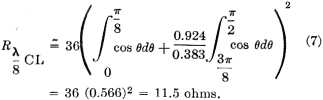
= 36 (0.566)2 = 11.5 ohms.
Bottom-Loaded λ/16 Monopole or λ/4 Monopole Folded Twice
Antenna Radiation Resistance
The cosine integral is broken down into four equal parts between 0 and
π/2 or 90
degrees. Two alternate parts are added and the other two are subtracted. The resulting
impedance, which is the same as that of a bottom-loaded sixteenth-wavelength monopole,
is
λ/32 Monopole Antenna Radiation Resistance
(Eight integrals)
Top- and Bottom-Loaded λ/8 Monopole Antenna Radiation Resistance (Fig. 5)
In this case the far-field factor is twice the cosine integral from 0 to
π/8. In
calculating the impedance, however, we must divide by the square of the cosine of
π/8 or 22.5
degrees, since we are feeding at a point 22.5 degrees from the current loop. This
is similar to the case considered in equation (5). Therefore,
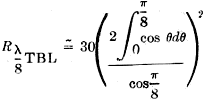
= 30 (0.830)2 = 21 ohms.
3λ/4 Folded Dipole (Fig. 7C)
The far-field factor for this case is found by calculating the difference between
the cosine integral from 0 to 3π/4 and the integral
from 3π/4
to 3π/2.
This figure is 2.414 and from this the impedance of the folded 3/4-wave dipole comes
out to be about 420 ohms.
* Asst. Prof. Research, Georgia Institute of Technology.
1 Editor's Note: As some readers may not he familiar with the terms used here,
the following may be helpful:
A "thin" antenna is one having a very large ratio of length to conductor diameter,
approaching infinitely-small diameter; practically, a wire antenna at low frequencies
is "thin" but a 10-meter beam element is fairly "thick." The thickness affects the
resonant length, radiation resistance, and sharpness of tuning.
"Antiresonance" is the same as parallel resonance; in the antenna case, it is
the condition that exists when a resonant antenna is viewed at a voltage loop.
"Charge" and "charge distribution" are equivalent to "voltage" and "voltage distribution."
The" far field" is the radiation field at a large distance from the antenna -
so far that the waves may be considered to be plane waves, and, of course, far beyond
the region where the induction field is of any consequence.
A "monopole" is one-half of a dipole; e.g., a grounded antenna or one in which
a ground plane is substituted for actual ground.
2 Lindenblad, "Television Transmitting Antenna for Empire State Building." RCA
Review, 3, p. 400, April, 1939.
3 Terman, Radio Enoineers' Handbook, McGraw-Hill Book Co., Inc., New York, 1943,
par. 11, sec. 11.
4 Jordan, Electromagnetic Waves and Radiating Systems, Prentice Hall, Inc., New
York, 1950, pp. 510-517.
5 Kraus, Antennas, McGraw-Hill Book Co., Inc., New York, 1950; particularly Chapter
5 and par. 13 of Chapter 14.
6 Kraus, "Multiwire Dipole Antennas," Electronics, 13, pp. 26-27, Jan., 1940.
Posted October 3, 2022
(updated from original post on 4/19/2016)
|