Loops vs. Dipole - Analysis and Discussion, August 1976 QST

Computer analysis in 1976 was a job performed on a corporate, university, or government mainframe. Radio Shack's (Tandy's) TRS-80 came out in 1977*, but it did not have the capacity to calculate and plot antenna gain charts like the one in this QST article. Yes, an ambitious programmer could write the code necessary to perform the double integrals presented in the article, but to do all the figuring needed to create all the graphs in Figure 4, the job would just about be finishing up today - and that's not too much of an exaggeration. For some reason the authors never mention what computer was used or where it was based. When I saw the title of "Loops vs. Dipole," I expected the loop to be round or square, but for analysis purposes it was modeled as a pair of parallel elements representing the horizontal components of a square loop antenna. Justification for omission of the vertical sides was that their contribution compared to the dipole horizontal elements would be negligible. Computation intensity would have been significantly greater if the sides were included. A round antenna would have been out of the question for this kind of analysis because of the mathematics required. Of course today (for the price of a week's worth of Starbucks designer coffees), running EZNEC on any modern PC would permit modeling of just about any conceivable antenna geometry in any environment (obstacles, ground conductivity, antenna height, etc.) in a matter of a few minutes. Someday soon, quantum computers will do the job in the time it takes to press and release the mouse button.

* The IBM PC was a bit more powerful, but it didn't arrive on the scene until 1981. The Commodore 64 debuted in 1982, and Apple's Macintosh came in 1984. I used all of them in their day, BTW.

This computer analysis shows how the quad earned its reputation as an outstanding DX antenna.

Fig. 1 - Models used for the computer survey of the loop (A) and dipole (B) antennas.

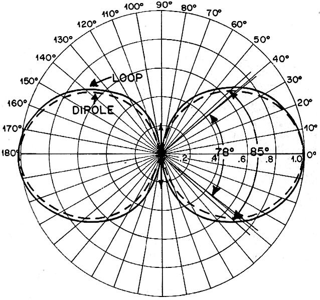
Fig. 2 - Normalized horizontal patterns for the loop and dipole antennas, all heights. For this and all following patterns, the solid line is for the loop.

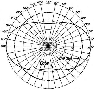
Fig. 3 - Free-space vertical patterns for both antennas. Maximum loop gain is 1.94 dB.

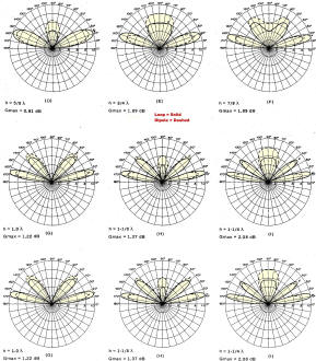
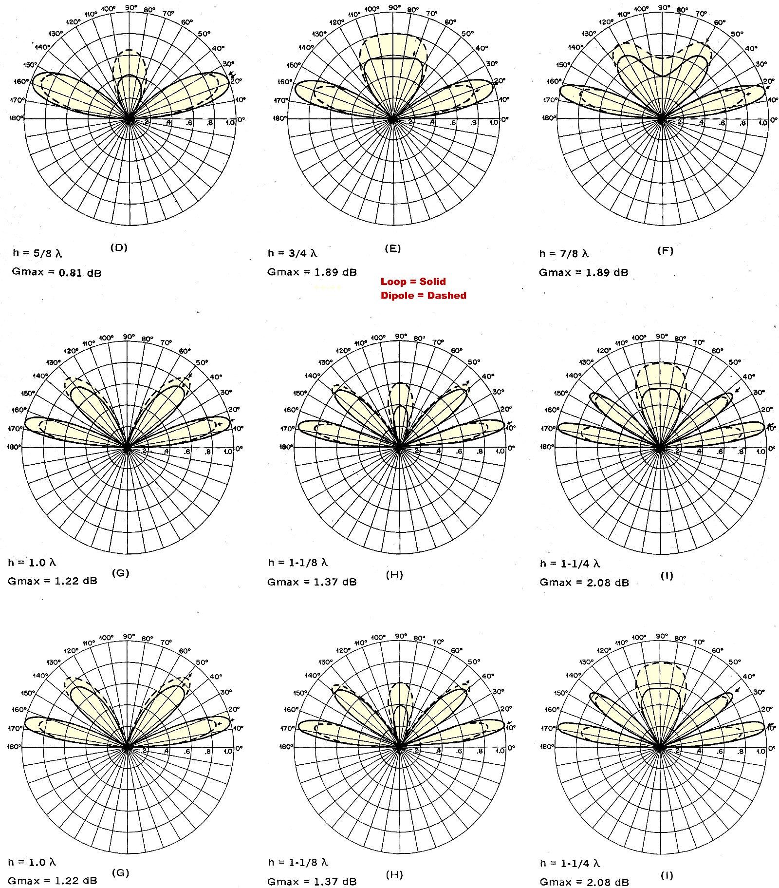
Fig. 4 - Vertical patterns and gains for the loop over the dipole antenna at various heights above perfectly conducting ground. Loop curves are solid lines. At low heights the gain for the loop is low and the radiation angles are high for both antennas, but the loop is superior in every case. Substantial improvement for the loop appears first at 3/4 λ, where its gain approaches the free-space value and its radiation angle drops below 20° for the first time.

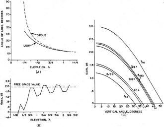
Fig. 5 - Comparisons of the performance of the loop and dipole in several categories of interest to the amateur. The vertical angle of the lowest lobe for the two antennas is given in A. Gain of the loop over the dipole at heights up to 2-1/4 f... is shown in B. Gain for the loop over the dipole at vertical angles up to 50° is given for various heights in C.

Over the years there have been many claims pro and con regarding the performance of full-wave loop antennas. Loops in diamond, square, circular, and hexagonal shape have been described. Unfortunately for prospective users, most of the comparisons have not been very analytical. Relative performance claims have often been based on differing models, assumptions, and measurement techniques. The loop's gain over a dipole is one fact about which there is disagreement. Lindsay¹ reported 2 dB, while Orr² reports 1.4. There have been other figures in between these two numbers.

A computer study of the loop-dipole question revealed that the disparity apparently results from the model chosen. If the current maxima are farther apart, as in a circular or diamond-shaped loop, the higher gain figure results. Our model attains the 2-dB figure, since more rigorous analytical and empirical information is available on that configuration.

Another curiosity concerns the loop's reputation as a good DX antenna. It does not seem reasonable to attribute this to a mere 1.5 to 2 dB of gain, which is barely distinguishable to the human ear, and Lindsay claims that the vertical angle of radiation is "essentially the same." Having the various contradictory facts, the authors decided to perform an analysis rigorous enough to uncover some of the misconceptions.

Information available to date has not extensively considered loops above ground, in direct comparison with dipoles above ground. Actually this is the only situation to consider, since with all ground-based hf antennas this is the case.

In order to model the loop antenna, only the major radiation component (horizontal) is considered. Fig. 1 shows the model for both the full-wave loop and the half-wave dipole. In the analysis the height above ground, H, is assumed to be that of the geometric center of the loop elements. Ground is considered ideal.

3) The drive currents in all antenna elements are adjusted so that the total radiated power from the antenna systems is equal.

4) The fields of both antennas are then plotted on the same graph for one height.

The comparative horizontal patterns of the loop and dipole are shown in Fig. 2. The plot represents horizontally polarized E-field intensity only, as it varies with azimuth angle. The loop is known to have small vertically polarized side lobes, but all vertically polarized components were omitted from the analysis and will not be discussed. As is apparent from the figure, the dipole has a slightly narrower 3-dB beam width approximately 78°, compared to 85° for the loop.

Fig. 3 shows the comparative free-space vertical patterns for both antennas. The dipole has the familiar isotropic pattern, whereas the loop has a "peanut" pattern resulting from some vertical-direction phase cancellation in the plane of the loop. The E-field intensity amplitudes shown on the graph may be directly ratioed for a true indication of relative power radiated at my vertical angle. For example, if the E-field values for zero degrees are taken, the maximum power gain of the loop over the dipole is found to be

This compares favorably with the 2-dB free-space gain figure reported by Lindsay for the circular loop, and substantiates that the simplified loop model used in the computer analysis approximates the correct free-space performance. Theoretical free-space conditions are interesting for examining ideal element radiation pattern comparisons but of primary interest to amateurs operating the hf bands are the effective patterns in the presence of ground.

Figures 4A through 41 show what happens when loops and dipoles are suspended at various elevations above perfectly conducting earth. At a quarter-wave above ground (Fig. 4A) the dipole radiates maximally straight up. The loop at the same height is better, giving a peak at about 45° and radiating substantially greater power than the dipole at lower angles. But by the standard way of comparing antenna gains (ratio of lobe peaks) we see that the dipole radiates a slightly stronger E-field straight up than the loop does at 45°, resulting in a loop-to-dipole gain (G_max) of -0.31 dB. As the elevation increases, the lobe angles decrease and a vertical null begins to form until at λ/2 above ground (Fig. 4C) a complete vertical null exists. At this elevation there is little difference between the peak lobe angles for either antenna (30° dipole vs. 27 loop), and the difference becomes even less as the height increases (Figs. 4D through 4I, and Fig. 5A). Continuing above λ/2, another vertical direction lobe forms, grows, splits, and nulls by 1.0 λ (Fig. 4G), and this process just continues with more height.

It is interesting to note that the G_max loop gain over a dipole does not become significant until 3/4 λ above ground, where it is up to 1.89 dB (Fig. 4E). Fig. SB shows how G_max varies with height, first nearing the free-space figure at 3/4 λ and seesawing on up with more height. This figure shows that the 2-dB gain of the loop over a dipole does not become available until the elevation gets to 3/4 λ but the reputation of the loop is for exceptional performance over a dipole especially at low elevations. This advantage does in fact exist if one ignores the lobe peaks and compares only the absolute field intensities radiated at each angle.

Using Figs. 4A through 4I to obtain relative field intensities radiated at various vertical angles, we get the set of curves plotted in Fig. 5C. At an elevation of only λ/4 it is evident that up to 3-dB more power is radiated at low angles by the loop than by the dipole. The reader is cautioned that this curve says nothing about where the lobe peaks are, but merely gives an indication of how much power the loop radiates at any specific vertical angle relative to a dipole at the same height. Heights of 3/8 λ, 3/4 λ, and 7/8 λ are also seen to be good for maximizing the low-angle advantage of the loop, whereas at λ/2, 5/8 λ, and 1.0 λ the gain is small but still significant.

As the figures have shown, the comparative performance of a loop vs. a dipole can vary rather widely with elevation. As every frustrated antenna engineer knows, the effective elevation of any antenna in the presence of objects such as houses, trees and power lines, and with varying ground conductivity, can be quite different from physical elevation. The most significant conclusion that can be drawn is that effective elevation is likely to differ from the physical height. Therefore, it would be a mistake for the amateur to place too much emphasis on achieving a precise elevation to realize a specific vertical pattern, unless true ground is known.

With real-world exceptions as they are, it is nevertheless possible to draw several meaningful general conclusions from the theoretical curves that have been presented here:

1) A full-wave loop antenna has a low-angle advantage over a dipole at all elevations. It is therefore a more effective DX antenna.

2) At angles below 10° the gain of the loop over the dipole never goes below 1.0 dB and may range up to 3 dB.

3) If the effective ground elevation of a particular installation is known with confidence, it may be predicted that λ/2 is particularly bad elevation for a loop in terms of advantage over a dipole.

4) The loop has a slightly broader horizontal pattern, but the difference is so small to be of little significance.

5) The vertical lobe peak angles are substantially different up to λ/2 height, and track closely at higher elevations .

1) In all real-world situations, the loop is somewhat unbalanced between top and bottom currents which causes the vertically polarized components of radiation to be greater.

2) This vertically polarized component may be a substantial reason for the loop's added advantage, especially during periods of marginal band conditions.

3) Two vertically stacked half-wave dipoles have the potential to out-perform the loop.

4) A one-wavelength horizontally polarized loop may have more gain in the diamond configuration than in the square. This is due to the current centers being separated by different distances and could account for the diversity of gains reported. Perhaps some interested reader would care to analyze this possibility further.

The horizontal electric field intensity E(Θ Φ) can be defined by the methods in step 4 of the computer analysis as

The equation is valid for both the loop and dipole antenna. Note from the model that H>D/2 in order to keep the bottom loop element above ground. D is 0.318λ to approximate Lindsay's model.

After calculating the electric field intensity at all points in a 1/8 sphere, the total radiated power is computed for each case at unit radius and unit space impedance, since the ratio of the absolute power is important.

For ease of plotting, all field intensities are again normalized to a maximum value of 1.0.

² Orr, "Antennas," CQ for January, 1974. Orr, All About Cubical Quad Antennas, Radio Publications, Inc., second edition, 1971, p. 16. Kraus, Antennas, McGraw Hill Book Co., 1950.

Loops vs. Dipole - Analysis and Discussion August 1976 QST

Loops vs. Dipole - Analysis and Discussion
August 1976 QST