Low-Frequency Narrow-Band FM, July 1947 QST

Narrow-band frequency modulation (NFM) was a relatively new technology in 1947, having been advanced significantly during World War II. Amateur radio operators were just getting their gear back on the air after having been prohibited from transmitting for the duration of the war (see "War Comes," January 1942 QST). Few were probably thinking about adopting and exploiting new modulation techniques, but for those who were and recognized FM as the path to the future of radio, QST published this fairly comprehensive treatment of both frequency modulation (FM) and phase modulation (PM). Mathematically, FM is the time derivative of PM. Both modulation schemes vary the carrier frequency in some proportion to the baseband signal. Author Byron Goodman provides some insight into the techniques.

F.m. and p.m. seem to be surrounded by more mystery than a.m. ever was. With experimental bands soon to be available at 3.9 and 14.2 Mc., interest in the subject should be increased considerably, so the following article is intended to clear up some of the hazy points. A simple p.m. modulator is described for those who want to get in on the ground floor.

Fig. 1 - Spectrum analysis of an a.m. signal. The unmodulated carrier is shown at A, modulation by a single audio frequency is shown at B, and modulation by two frequencies is represented in C. There is a single pair of sidebands for each modulating frequency, and the sidebands are removed from the carrier by that frequency.

Now that narrow-band frequency (and phase) modulation may soon be permitted in portions of the 3.9- and 14-Mc. bands, this seems like a good time to look at some of the points that have not been covered in recent issues of QST. There seem to exist several popular misconceptions of just what the modulated carrier of an f.m. or p.m. signal looks like and acts like, and it is the purpose of this article to attempt to dispel these ideas and replace them with clearer pictures.

Everyone is familiar with pure amplitude modulation - a simple picture of the distribution of energy in the spectrum of an a.m. signal is shown in Fig. 1. The carrier frequency is represented by a single vertical line, as in 1-A. If the carrier is modulated by a single frequency, F, of sufficient amplitude to produce 100% modulation, frequencies called "sidebands" are developed on either side of the carrier, with an amplitude equal to one-half the carrier amplitude as in Fig. 1-B. They are spaced in frequency from the carrier by the amount in cycles equal to the modulating frequency, as indicated by + F and - F, relating to the carrier frequency. If the modulating power is made up of a complex wave that can be resolved into two frequencies, as in Fig. 1-C, sidebands occur for each of the two components of the modulating frequency. Speech is a complex form that is practically always made up of two or more frequencies. However, the important thing to remember about a.m. is that for each modulation frequency, there exists a single pair of corresponding sidebands, and no more. The simple representation in Fig. 1-C does not necessarily take into account the relative phase of the modulating-frequency components, but it is adequate to consider that the sideband amplitudes never exceed half the carrier amplitude for 100% modulation. Further, when a sideband on one side of the carrier is at a maximum, the corresponding sideband on 'the other side is also at maximum.

A simple phase-modulator unit that can be used to drive the average crystal-oscillator stage. Receiving tubes are used throughout, and the output is about one watt. The black shield houses one of the coils. Power plug and gain control are at the rear.

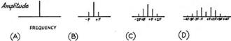
Fig. 2 - Spectrum analysis of an f.m. or p.m. signal. The unmodulated carrier is shown at A, and modulation by a single frequency is shown in B, C, and D. B corresponds ,to a low degree of modulation, C and D show what takes place as the modulation is increased. All sidebands are spaced an amount equal to the modulating frequency. Note that the amplitude of the carrier decreases as the modulation is increased.

Frequency and phase modulation do not lend themselves to such simple pictures. It is generally understood that frequency modulation is obtained by changing the carrier frequency at the frequency of the modulation, and the greater the amplitude of the modulation the greater the frequency change, or deviation, from the mean carrier-frequency. Phase modulation, on the other hand, is obtained by shifting the phase of the carrier frequency at the modulation frequency, and the greater the amplitude of the modulation the greater the phase change. With a little thought it can be seen that as the phase of the carrier is changed, by speeding up or slowing down the r.f. alternations during the audio modulation cycle, the frequency of the carrier must change at the same time, since more or fewer alternations than normal must occur during the speeding-up or slowing-down process. Hence f.m. and p.m. are similar in that the carrier frequency is changed during the modulation cycle.

Then it starts to get complicated! When a single tone is used to modulate a carrier in either phase or frequency, not a single pair of sidebands results, as with a.m., but theoretically an infinite number of sidebands develops. The magnitude of the sidebands depends upon the amplitude of modulation, with the sidebands close to the carrier being the larger and the remote sidebands existing only theoretically for all practical

purposes. To examine the procedure in an orderly fashion, assume a carrier modulated by a single 1000-cycle tone. With very little modulation, only the first pair of sidebands have any significant amplitude, and the picture looks similar to the one for low-percentage amplitude modulation. As the degree of modulation is increased, the second and third and higher-order sidebands begin to be significant, as shown in Figs. 2-B, 2-C and 2-D. Notice that the sidebands occur at regular 1000-cycle intervals. This is a significant point, since many seem to believe that f.m. (or p.m.), can be made to occupy less spectrum space than a.m. by keeping the frequency swing low. 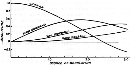Such is not the case - the instant any modulation is applied to the carrier, sidebands exist removed from the carrier by the modulation frequency. Fig. 3. shows how the amplitude of the sidebands varies with the index of modulation - for some degrees of modulation, some sidebands disappear and so does the carrier. Also, some pairs of sidebands will be out of phase with each other for high degrees of modulation.

Fig. 3 - Showing how the amplitude of the sidebands of an f.m. or p.m. signal varies as the modulation is increased. If the curves were extended for greater values of "degree of modulation," it would be seen that the carrier value goes through zero at several points, as do the various sidebands. Amateur n.f.m. and n.p.m. should be confined to a degree of modulation equal to 0.5 or 0.6, so the additional sidebands are not significant.

What we have elected to call "degree of modulation" in the above discussion is more correctly known as the" modulation index." The modulation index is defined, for f.m., as the ratio Δƒ/ƒ where Δƒ is the frequency deviation and F the highest modulation frequency. For p.m., it is defined simply as the phase change, in radians (one radian = 57.3 degrees). The curves in Fig. 3 apply to either f.m. or p.m., if the modulation index as described above is substituted for "degree of modulation."

The definition of modulation index helps to clarify the distinction between f.m. and p.m. and how their audio characteristics differ when rectified by the same detector system. In an f.m. system, for example, a modulation index of 2.0 means that the maximum deviation divided by the highest modulation frequency is equal to 2.0. If the top audio frequency is, for example, 5000 cycles, then the maximum deviation will be ± 10 kc. The f.m. transmitter with an index of 2.0 and a top audio frequency of 5000 cycles will deviate ± 10 kc. for full modulation at any audio frequency below 5000 cycles. Any greater deviation doesn't mean "overmodulation" as we know it for a.m., but simply that the signal can no longer be described as having an index of 2.0. If the detection system is designed to give maximum output for a deviation of ± 10 kc., then a greater deviation will result in distortion in this detector, and it might be described as "overmodulation," but only for that particular detector. Whether the modulating signal is 100 or 5000 cycles, maximum undistorted output from the detector will be obtained when the deviation is ± 10 kc. in either case. Note that this represents a modulation index at 100 cycles of 50. If Fig. 3 were extended to values of index ("degree of modulation" in sketch) of 50, it would be found that the total number of significant sidebands would be multiplied enormously. But with the modulation frequency of 100 cycles, these sidebands are now only 100 cycles apart, and actually the significant sidebands (less than 30 db. down) do not extend out as far as the fewer but more widely separated sidebands of the 5000-cycle modulation frequency. It is therefore readily apparent from the examples in this discussion that, with f.m., the modulation index gives rather incomplete information on the bandwidth unless the highest audio frequency is also specified.

In p.m. and any given modulation index, the number and amplitude of the sidebands are exactly the same for any single modulation frequency, since the index in this case is only the number of radians of phase swing either side of zero required to give the phase modulation. However, the sidebands are separated by the modulation frequency, so a low frequency of modulation will result in a narrow bandwidth and a higher modulating frequency will cause the signal to occupy more spectrum space. If the index is low (0.5 or less), so that only the first sidebands can be considered as significant, this gives a spectrum picture quite similar to that for a.m. Fig. 4 illustrates the comparative spectrum space occupied by f.m. and p.m. signals for different modulation indices and modulation frequencies. The p.m. pictures show immediately why pure p.m. received on an f.m. detector will be lacking in "lows," since the f.m. detector requires that modulations of equal intensities but different frequencies have roughly the same deviations. The condition can be corrected, of course, by attenuation of the "highs" at the transmitter or receiver. The latter is generally more convenient, since most receivers have a "tone" control that can be cranked over to give the necessary attenuation of the higher frequencies.

One point worth noting about p.m. is the fact that it does not necessarily require a long string of frequency multipliers following it in order to obtain a usable index. Readers familiar with the Armstrong system of f.m. know that p.m. is used at a low level and converted to f.m. Such a system does require considerable multiplication, for reasons that will be described, but this is only because f.m. is the desired end product. It is not impossible to obtain an index of 0.5 in p.m. without any multiplication, and, indeed, this seems to hold the most promise for simple work on the 75-meter band.

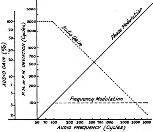
Reference to Fig. 5 will show why f.m. obtained by phase modulation requires so much multiplication. For a p.m. signal, plotting deviation vs. modulating frequency gives the solid line sloping up from the origin. Since f.m. requires nearly the same deviation for all modulating frequencies, it is necessary to modify the audio characteristic, as shown by the dotted line. This results in the f.m. characteristic indicated by the dashed line, but note that it reduces the deviation to that obtainable through p.m. at the lowest usable audio frequency. To minimize distortion, the phase modulation is held down to a low level anyway, and the total result is a very low modulation index at the control frequency. Such technique is not necessary in amateur work, and hence p.m. looks good for our low-frequency bands. Phase modulation suffers in its ability to reject noise, but this is not under discussion, although it is of course a big point in the Armstrong system, and accounts for the use of f.m. and a high index.

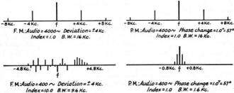
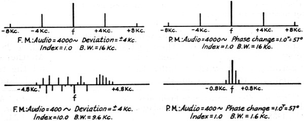
Fig. 4 - A comparison of the bandwidths of f.m. and p.m. signals for different modulation frequencies. A modulation index of 1.0 and an upper frequency limit of 4000 cycles are assumed. Note that the sketch for f.m. with an index of 10 (lower left) shows the relative phase of the sidebands. Bandwidths are based on neglecting sidebands down more than 30 db.

Fig. 5 - The necessary audio correction (dotted line) to correct a p.m. characteristic (solid line) to f.m. (dash line). Note that this limits the resultant f.m. deviation to the highest uncorrected p.m, deviation. This is the principle used in wide-band f.m. transmitters, but it is not necessary for amateur work.

It is important that one more point be clarified in this discussion. The pictures given for single-tone f.m. or p.m. show a rather discouraging bandwidth for any narrow-band application, if exactly the same condition were to hold for complex modulation by two or more frequencies. However, when a complex wave is used to frequency - or phase-modulate a carrier, the resulting sidebands are not the same as would be obtained by superimposing the pictures of modulation by the component tones. The existence of the side-bands in f.m. or p.m. always results in the reduction of the carrier-frequency amplitude (see Figs. 2 and 3), and the total energy always remains the same. If two sets of sidebands exist, corresponding to two modulation frequencies, both of these sets of sidebands draw from the carrier, and the resultant effect is to reduce the amplitude of the sidebands, since the carrier sets the limit on total available energy. For this reason, a single audio frequency will yield higher-order sidebands than will a complex wave of the same amplitude. This means that a single tone applied to an f.m. or p.m. signal may show several sets of sidebands, while voice modulation of the same amplitude will not show as many. As a result, speech occupies less channel space than a single tone of the top frequency existing in the speech for a given modulation index.²

Another point that is often confusing is what happens to f.m. and p.m. signals at the harmonic frequencies of the carrier. At first glance, one might think that, if a carrier is frequency-modulated at its fundamental by a 1000-cycle tone, to give a pair of sidebands removed from the carrier by 1000 cycles, then the carrier and the sidebands would have harmonics, and so the sidebands would move out from the carrier at the harmonic frequencies. However, this is not the case, any more than it is with a.m. Unfortunately, there is no simple physical picture that can be given of the process of modulation of any type. We all know that sidebands are generated under modulation, and it can be shown readily by mathematics that the sidebands will appear. We can show the existence of the sidebands with a "spectrum analyzer," but they just seem to be something we have to accept on the basis of mathematical and practical proof. It isn't too many years since the "great sideband controversy" raged between the English and American engineers, the English holding that sidebands existed only in the mathematics.

The harmonics of the carrier result from distortion of the carrier in some nonlinear element, such as a vacuum tube. But the sidebands are a result of the operation performed on the carrier (a change in amplitude, frequency or phase). The change of frequency or phase is multiplied in direct proportion to the frequency multiplication generating the carrier harmonic frequency, but the sidebands set up are the same as those produced by direct modulation of a carrier fundamental but with the greater index of modulation. Hence in most f.m. and p.m. work it is customary to do the modulation at a low frequency and frequency-multiply until the necessary index is obtained.

It will be necessary for any operator using narrow-band f.m. or p.m. to check his transmissions and to be sure that his signal is occupying no more spectrum space than an a.m. signal, in keeping with the definition of n.f.m. The future of f.m. and p.m. in the amateur bands depends on those who use it during the trial period and, since it is proving to be such a boon to those heckled by BCI, it would be unwise and unfair to jeopardize its future by giving it a bad name on the air - and with the FCC monitoring stations. For this reason, it is the duty of every user of f.m. and p.m. to do his best to insure that his equipment is properly checked and monitored. Unfortunately, this is not a simple problem, and no such clean-cut solutions as exist for a.m. are known at the present time.

In the case of wide-band f.m., it is possible to apply single-tone modulation and increase the modulation until the carrier disappears.³ This corresponds to an index of 2.4 for the first disappearance of the carrier, and 5.5 for the second. This is not a convenient method, however, for a station operating on 14 or 28 Mc., unless the operator has access to stable receiving equipment at 56 Mc. or some such high harmonic frequency. One would then establish the audio level required to give the necessary deviation, knowing that the index would be divided by the order of multiplication, and then keep his modulation below this level, by means of a 'scope or some other audio-level indicator. Figuring on an operating index of 0.6 at the operating frequency, this method would require a 56-Mc. receiver to check a 14-Mc. signal and a 112-Mc. receiver to check a 28-Mc. n.f.m. transmission, either one with excellent frequency stability and good selectivity. A 3.9-Mc. signal can be checked, of course, by a receiver capable of tuning to 15.6 Mc.

Another method, which is unfortunately beyond the reach of most amateurs, is to use a special "spectrum analyzer" designed for n.f.m.

This is an instrument similar in principle to a panoramic receiver, but in this case it requires a few refinements such as a crystal-filter i.f., a slow sweep rate, and a long-persistence screen (to handle the slow sweep rate). Such a device would make an excellent club project, but it is hardly likely to become standard ham-shack gear. However, it is quite possible that it will be the sort of thing the FCC monitoring stations will use for checking amateur n.f.m. transmissions, since it offers an instantaneous picture of the bandwidth. This is no hardship on the n.f.m. gang, however, because the same instrument turned on maladjusted a.m, signals would also tell the sad story about them.

Since the precise methods are involved and expensive, we must fall back on something a little more simple and less complicated. One redeeming feature of n.f.m. is that one can listen to it as it will sound on the air without turning on the whole transmitter, and this provides an excellent opportunity to do all the testing without putting the signal into an antenna. By tuning in the harmonic of the n.f.m. unit on the band where operation is to take place, one can get a rough check on the bandwidth by noting how much room the signal takes in comparison with a.m. signals on the same band. The most precise method available to the average amateur to measure the bandwidth is to use his communications receiver and its crystal filter as a sort of "poor man's spectrum analyzer." If the receiver is accurately calibrated in kilocycle steps - which means that the absolute calibration can be off but the kilocycle divisions accurate - or if a suitable calibration chart can be made to find out how many dial divisions per kilocycle exist at the operating frequency, the problem is fairly simple. The receiver must be stable, of course, and any measurements should only be made after a suitable warm-up period. Suppose, for example, that one is setting up his f.m. or p.m. signal in the 14-Mc. band. The oscillator and possibly one or two following stages are turned on, to give a reasonable signal in the receiver tuned to 20 meters. The signal level should be equivalent to an average signal in the band, as judged by the S-meter, and it may be necessary to short the input of the receiver to get it, unless the oscillator and other stages are operating at a low power level. The receiver crystal filter is set to its sharpest position, the b.f.o. is turned on and the a.v.c. turned off. It may be necessary to reduce the r.f. gain slightly, to avoid overload of the receiver. Tune the carrier on the peak of the crystal and set the b.f.o. for the usual beat note, around 500 or 600 cycles. If the receiver is accurately calibrated, either by the manufacturer or by the operator making a calibration curve, detune it exactly 3 kc. If the calibration isn't available, it will be necessary to modulate the f.m. or p.m. unit with a 3000-cycle tone, which can be obtained from an audio oscillator built or borrowed for the occasion. The 3000-cycle modulation will cause sidebands to appear on either side of the carrier, spaced by 3000 cycles, and one of these will serve as a reference point. The amplitude should be kept low, so as not to introduce more than one pair of detectable sidebands.

After the receiver setting is established 3 kc. off the carrier frequency, talking into the microphone and experimenting with various voice levels will give some level at which the voice is heard to splash over occasionally. This represents the upper limit of modulation level that should be used. Once the proper level has been established, it can be monitored by a 'scope or other voice-level indicator connected in the audio amplifier ahead of the frequency or phase modulator, unless one is willing to run the risk of depending upon the setting of the gain control and one's memory of his voice level, bearing in mind his responsibility not to give n.f.m. a bad name, or the FCC a chance to tag him. There is nothing simple that can indicate directly from the carrier, as in a.m. work, since a properly-adjusted f.m. or p.m. transmitter will be accompanied by no amplitude changes under modulation.

If the operator's voice is naturally high-pitched, the 3-kc. figure may be slightly unfair, and perhaps 3.5 or even 4 kc. is a more reasonable limit. However, there aren't very many necessary components existing in normal speech that run this high, if there are any, and they are just as likely to be introduced by distortion in the audio amplifier or modulator. The best practice, as in a.m., is probably to limit the upper response of the audio amplifier to the useful frequencies below 3 or 3.5 kc., by means of suitable filters.

During the past few years, a number of different types of phase modulators have been described in the literature. The new Raytheon cascade-modulation system is interesting, but it requires a number of stages and the tuning procedure does not lend itself too well to rapid frequency change, as is often required in amateur work. Other systems using balanced modulators in one form or another are at a disadvantage mainly because their apparent complexity will frighten a few potential customers for p.m., although they are actually quite satisfactory in every respect.

One of the attractive things about p.m. is that it can be applied to the transmitter at some point other than the oscillator, without any alterations that might impair the frequency stability. Until we have quite accurate methods for measuring and insuring bandwidth of f.m. transmissions, it seems highly desirable to avoid the use of direct reactance modulation on the oscillator to obtain an f.m. signal. This fact alone makes p.m. a natural for amateur use. Also, it is more difficult to obtain a high index of modulation with p.m. than with f.m., so the bandwidth is inherently more limited.

The simplest phase modulator we have been able to find is one suggested in Mr. Hund's book.⁵ The author suggests using a reactance modulator across the tuned plate circuit of a driven r.f. pentode amplifier. When the reactance modulator changes the tuning of the circuit in accordance with the modulation, the phase angle of the effective tuned circuit is changed and hence the phase of the voltage developed across it. Since the phase change across a tuned circuit of Q = 10 or higher is fairly linear for a range of ±25°, all that is required is a reactance modulator capable of detuning the tuned circuit the necessary amount. Assuming a Q of 20 for the circuit, an angle of 26.5° is obtained when the detuning is an amount equal to 1/4Q - RF Cafe

. This works out to be Frequency formula - RF Cafe

= 0.04875 Mc. = 50 kc. approx. A Q of 20 will be obtained at 3.9 Mc. with a total tank capacity of 50 μμfd. and an effective parallel resistance of 16,300 ohms (from Q = 2πƒRC). A change of ± 1.2 μμfd. will swing the 50-μμfd. tank ± 50 kc., and this is easy to obtain with a reactance modulator. From the design equations,⁶ this can be obtained with a reactance modulator using an inductive element of 2.5 mh., a resistive element of 0.5 megohm and a mutual conductance change of ± 240 μmhos. This is a reasonable range for almost any of the better receiving-type pentodes.

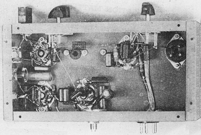
Fig. 6 - A simple phase-modulator unit.

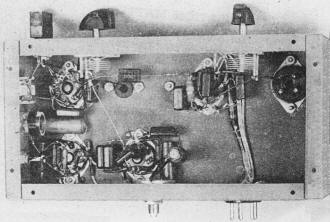
A view under the chassis of the phase modulator. The Tri-tet cathode circuit is mounted on the side of the chassis near the microphone connector.

An experimental model was built and is shown in the photographs. The wiring diagram, shown in Fig. 6, shows how simple the unit can be. A 6SJ7 speech amplifier builds up the signal from a crystal microphone sufficiently to give enough swing for the reactance modulator. A gain control, R₅, allows the gain to be reduced when the transmitter output is on 14 or 28 Mc., since the multiplied modulation index at these frequencies might be too high. The reactance modulator is slightly different than those previously described in that it uses an inductance-resistance divider, RFC₁R₆, to obtain the quadrature current rather than the more usual condenser-resistor combination. The principle, however, is practically the same, and it requires no elaboration here.

A Tri-tet oscillator is used, with straight-through operation; i.e., the plate circuit is tuned to the crystal frequency. Since this type of operation requires a well-screened tube, the 6SK7 was selected. The effect is the same as if a separate crystal-oscillator tube were used to drive an amplifier, since the plate-circuit tuning or loading has no effect on the crystal oscillation. This is important if one is to obtain pure phase modulation. If VFO were to be used, the VFO would feed into a tuned circuit between grid and ground of the 6SK7, and the tuned cathode circuit would be replaced by a bias resistor and by-pass condenser. In the unit shown, the tuned cathode circuit is resonant around 4.5 Mc. Its tuning will affect the amount of oscillator output slightly, but the major control of output is the value of oscillator screen voltage. This was made convenient to adjust in the model by bringing out the lead separately (marked "screen") and running it to the regulated 150 volts through an adjustable resistor. The value isn't critical, and several fixed resistors are all that is necessary to make the adjustment. The oscillator output must be adjusted to avoid overdriving the amplifier. The inductance L₂ is shielded to avoid self-oscillation in the amplifier, and the plate by-pass condenser, C₁₆, is mounted across the tube socket to shield the grid and plate pins from each other.

Since this particular unit is only a model and will probably not fit too well into anyone's ideas about how such units should be constructed, only the tuning details will be included. The operator with VFO can use the circuit by making the oscillator changes mentioned earlier, and the station requiring more power output from the unit will require additional power stages following the 6SG7 amplifier. The output of this little unit is enough to light a small pilot lamp, representing about one watt of power, enough to drive the usual crystal-oscillator stage. The direct substitution of larger tubes throughout the unit is not recommended, unless a well-shielded tube like the 802 is used, since one is likely to encounter the usual difficulties with feed-back if beam tetrodes are used.

The first step in putting the unit in operation is to adjust the crystal oscillator. With the screen of the oscillator connected directly to the 150-volt source, and with normal voltages on the rest of the unit, adjust the cathode-circuit condenser, C₉, until the crystal oscillates. A 0-1 milliammeter between the bottom of R₁₁ and ground will serve as an output indicator, and a receiver should be used as an additional check on the signal. When oscillation of the crystal has been checked, add resistance in the oscillator screen lead until the grid-current reading reaches a low value, of around 0.1 ma. or less. It should still be possible to swing the tuning of C₁₁ without throwing the crystal out of oscillation or even affecting the frequency. If it can be thrown out of oscillation, readjust C₉ or reduce the value of the screen-dropping resistor. In the unit shown, 0.2 megohm could be connected in the screen lead without stopping crystal oscillation.

If a VFO is being fed into the unit, the screen voltage of the 6SK7 should be reduced until the drive on the 6SG7 amplifier is as specified for crystal operation.

Using a small lamp load or the grid current of the stage the 6SG7 is driving, resonate the output circuit L₃C₁₇. If it tunes broadly, it probably indicates that the stage is being overdriven, or that the 6SG7 is oscillating, although no trouble with oscillation was encountered in this unit. The modulated circuit, L₂C₁₁, will tune broadly because it is loaded by R₁₁, but it should be centered on the broad resonance peak or otherwise the modulation will fall off.

Talking into the microphone and monitoring the signal on 14 Mc. will give you a check on the modulation, in the manner described earlier in this article. It will be found that more than enough modulation can be obtained for 14 Mc. when using an 80-meter crystal, but on 3.9 Mc. the best reception is obtained when using crystal-filter reception methods, as outlined previously.⁷ For 3.9-Mc. work, it would probably be better to do the modulating at 1.95 Mc.

No great claims are made for the unit, except that it is a simple thing to get going and it will enable all of us that are interested to take advantage of the opening of the lower-frequency bands to p.m. Somewhat greater swing can be obtained by increasing the value of R₁₁, and this might be necessary if a low-output microphone is used. If listeners report "no lows," explain that you're using p.m. and suggest that they crank up the tone control on their receivers. However, a cheap crystal microphone may have poor low-frequency response, so the fault may be in your own equipment if you are using a bargain microphone. Good practice would indicate a low-pass filter ahead of the reactance modulator, to limit the high-frequency response and consequently, the bandwidth, and such a filter could be put in the circuit ahead of the gain control.

1 The information for these sketches and for Fig. 2 was obtained from Hund's Frequency Modulation, McGraw-Hill Book Company, an excellent text for further study of the subject.

2 Crosby, "Carrier and Side-Frequency Relations with Multi-Tone Frequency or Phase Modulation," RCA Review, July, 1938.

3 Crosby. "A Method of Measuring Frequency Deviation." RCA Review, April, 1940; also: Grammer, "Getting on 56-Mc. F.M.," QST, June, 1940.

Low-Frequency N.F.M.July 1947 QST

Low-Frequency N.F.M.
July 1947 QST