Artificial Delay Lines |
|
There are probably few baseband and IF delay lines these days that are constructed from a chain of inductor-capacitor (LC) sections as described in this 1953 Radio-Electronics magazine article. SAW and MEMS devices are the more likely choice for many reasons including cost, weight, and volume savings. The preferred implementation of measured delays nowadays would be in software after sampling with an analog-to-digital converter (ADC). There are still applications for coaxial delay lines such as phase matching or adjustment between system elements, and many companies offer custom designs with delay precision in the tens of picoseconds. I once worked on part of a VHF/UFH transceiver unit that used precise lengths of coax cable as part of a signal cancellation circuit for enabling multiple radios to function in close proximity. I was not the designer, but did spend a fair amount of time building, measuring, and adjusting the cables, which interfaced between the antenna and a software programmable phase canceller built from Ls and Cs. I have to admit I never did fully understand how that cancellation system worked its magic, but it did work well ;-( The X-band precision approach radar system I worked on in the USAF used a mercury delay line in the moving target indication (MTI) cancellation circuit. I probably didn't fully understand how it worked either. Fortunately, in both instances my only need was to be able to adjust the system to function properly. Delay Lines Have Many Electronic Applications
One way of constructing a multisection delay line. The adjacent coils are mounted at an angle, to reduce coupling. Construct yours from low-pass filters made with L-C components By R. C. Paine In radar a distant plane is detected by radio waves reflected from the plane as a radio echo, just as sound waves reflected by a distant cliff create an acoustic echo. The audible echo is produced because the time it takes for the sound to travel out to the cliff and return is perceptible to the human senses. Even the radio echo requires a definite time for the waves to reach the target and return, though this time is measured in microseconds. Radio waves travel through free space at the speed of light - 300,000,000 meters per second, or about 984 feet per microsecond. Distance can be determined by measuring the time of arrival of the reflected waves.
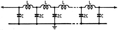
Fig. 1 - An artificial transmission line assembled from identical low-pass-filter sections linked end to end. Input and output capacitors are each half the value of the internal capacitance elements.
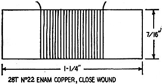
Fig. 2 - One of the line-section coils.
Fig. 3 - Checking voltage distribution along the artificial transmission line.
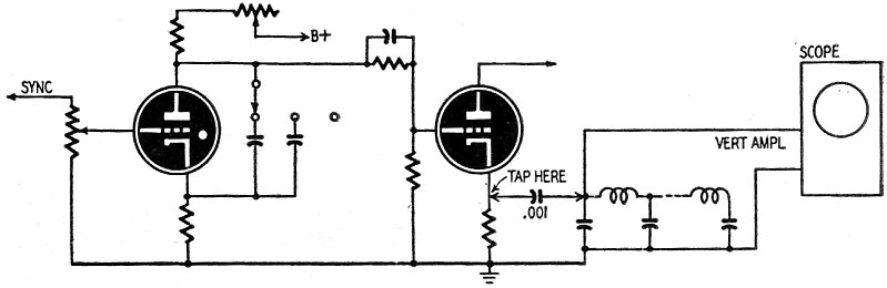
Fig. 4 - Using the oscilloscope sweep as a pulse source for checking line characteristics. Reflections are observed and counted on the scope screen for different values of line-terminating resistance. The time of travel of waves between points may be referred to as "delay time." For many purposes, such as range measurements in radar and loran, and storing information in calculating devices, circuits which produce definite time delays are required. Theoretically, it would be possible to use radio transmission line for delay circuits, because the speed of radio waves in ordinary transmission cable is less than in free space; but this approach is not very practical, since thousands of feet of line would be required to produce appreciable delay times. To avoid the bulk of long transmission-cable delay lines, artificial transmission lines with lumped constants are constructed. Over a limited frequency range, a relatively compact network of coils and capacitors can simulate the distributed series inductance and parallel capacitance of a long transmission line. The more sections such a line has, the more nearly it duplicates the performance of a uniform line. These artificial transmission lines are often used as delay lines to retard electrical impulses for a definite time (measured in microseconds, or millionths of a second) between points in a network. Such lines are used in radar and navigation systems, computing machines, and many other instruments. The characteristics of a delay line are usually studied with pulse generators and special complex oscilloscopes. An experimental line, however, is easily constructed and its delay characteristics can be observed readily with an ordinary oscilloscope. A delay line is shown schematically in Fig. 1 as a series of pi sections. The end capacitors have a value C, but the intermediate capacitors combine two parallel C values into a single one. One such line constructed by the author consists of thirteen sections and is shown above. The coils and capacitors are arranged in line and connected to a common grounding strip. Adjacent coils are tilted right and left at an angle of 45° to minimize coupling between them. The inductances L are wound on paper forms 7/16 inch in diameter and about 1 1/4 inches long, as shown in Fig. 2. They are wound with about 28 turns of No. 22 enameled wire and have an inductance of 5 microhenries. The end capacitors, C, are nominal 0.001-μf units selected for an actual value of 925 μμf each. The internal capacitors were selected from 0.002-μf units for a measured value of 1850 μμf. The line has a characteristic impedance of about 50 ohms. That is, when it is terminated by this value of resistance all the energy that reaches the end of the line is absorbed by the load, and reflected waves are suppressed. This artificial line has a time delay of about 1.15 microseconds. The time required for an impulse to go out and return as a reflected wave on this line is 2.3 microseconds. This is equivalent to quarter-wave-line resonance at 435 kilocycles, or half-wave resonance at 870 kilocycles. Resonance on this line can be demonstrated in an interesting manner. It can be driven by an oscillator operating at 870 kc. The line is coupled to the oscillator by a loop of a few turns connected across its input end as shown in Fig. 3. Its far end is short circuited. Voltage and Current Ratios The current distribution due to standing waves is at a minimum in the center of the network, but gradually increases to a maximum as each end is approached. Correspondingly, the voltage across each coil at the center of the network is low, but increases towards the ends of the line. A small flashlight bulb with probe terminals may be used to bridge each coil in succession. Near the center of the network the lamp glows dimly or not at all, but at the ends it lights brightly, and - unless caution is observed - it may even burn out. To check the reflected waves in a line we feed in a pulse and observe its progress on an oscilloscope. By using the return sweep of the oscilloscope for the initial pulse the two functions are combined and synchronized automatically.
Fig. 5 - Reflected signals on an open-ended line are in phase with the input, and cause the voltage to rise at the input end with each new reflected wave.
Fig. 6 - A line terminated in less than its characteristic impedance creates multiple reflections which are damped out eventually by the line resistance.
Fig. 7 - Perfectly terminated line has no reflections. All energy is dissipated in the load connected across the far end. A portion of the sweep circuit of a typical scope is shown in Fig. 4. The input of the delay line is connected through a 0.00l-μf capacitor to the out-put of the sweep amplifier (a cathode follower in this case) and also to the vertical input terminals of the same scope. With other scopes it may be necessary to connect to different points in the horizontal sweep circuit, but a small capacitor should always be used for coupling. This capacitor, together with the low input impedance of the delay line, differentiates the retrace of the saw-tooth sweep wave and produces a sharp pulse for exciting the line. Mismatched Impedances When the delay line is connected in this manner, its input or "near" end is terminated by the relatively high impedance of the scope input amplifier. Thus, waves reflected from the open-circuited far end are rereflected from the near end. Successive reflections take place until the energy of the original pulse is dissipated in the resistance of the line. If the far end of the line is open, or terminated in a high impedance, reflected waves are of the same polarity as the incident waves at each end and build up the voltage at each reflection (See "Transmission Lines Simplified," by Hector E. French, in the October, 1952, Radio-Electronics). This is shown in the oscilloscope photograph Fig. 5, in which the line is terminated by a 500-ohm resistor. A carbon or "metallized" resistor should be used for the termination because of its negligible inductance. An inductive termination would upset the delay-line constants. When the far end of the line is terminated by a low impedance or short circuit the polarity of the reflected wave is not the same as the incident wave at that end. This results in alternate recurring waves being reversed at the near end. This is shown in Fig. 6, in which the line is terminated in a 10-ohm resistor. The value of the terminating resistance can be varied until the observed reflections are reduced to minimum. At this point the load is equal to the characteristic impedance of the line, the incident wave is completely absorbed at the far end, and no reflections take place. This is illustrated in Fig. 7, where the 50-ohm terminating resistor is thus shown experimentally to be equal to the characteristic impedance of the line. Delay Time The delay time of the line can be estimated from the frequency of the oscilloscope sweep and the number of reflections as indicated by the total number of positive or negative peaks in Fig. 5. In this case the peaks (including one on the dim return trace) add up to nine. The frequency of the scope sweep was checked against an audio oscillator and found to be about 48,000 cycles, or 21 microseconds per sweep. This value divided by 9 gives 2.3 microseconds for each complete reflection, or transit in both directions. The observed delay for one way is thus 1.15 microseconds. Delay lines of different properties can be designed by using the formulas for uniform lines. Thus the characteristic impedance Z0, in ohms, is equal to 1,000√(L/C), where L is in microhenries and C is in micro microfarads. The total delay time is equal to the number of sections multiplied by √(L/C)/1,000. These formulas for uniform lines are approximately correct for lumped multi section lines. In the line described above the calculated values are Z0 = 1,000√(5/1,850) = 52 ohms and t = 13√(5/1,850)/1,000 = 1.25 microseconds. These calculated values compare favorably with the corresponding experimental values, Z0 = 50 ohms and t = 1.15 microseconds.
Posted February 28, 2019 |
|