|
As quoted in this 1954
Radio & Television News magazine article about analog[ue] computers as
compared to digital computers, "Add two and two. Coming from an analogue computer,
the answer would most likely be, 3.999 or 4.001." While that is a true statement,
there is one important feature that an analog computer had over digital computers
of the era: once initially set up with a transfer function, outputs were nearly
instantaneous as the input was varied over a range of values, whereas a digital
computer could take quite a bit of time to crank through involved mathematical equations.
Performing tasks such as computing aircraft flight paths and other sequential operations
was the analog computer's forte. If you needed to calculate exact values for atomic
research or cryptographic code cracking, that was and still is the domain of digital
computers.
See also
Mr. Math Analog Computer.
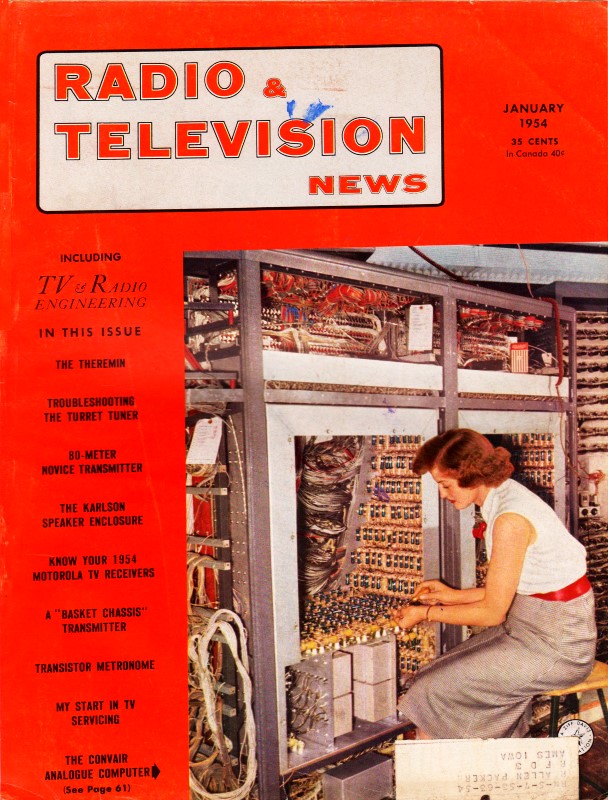
The Convair Analogue Computer
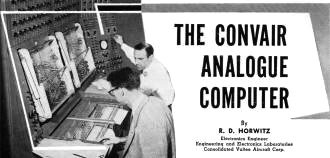
Fig. 1. The "Convair" analoque computer in operation. Two
problem patchboard stations in normal operating position are shown in one-half section
of the dual computer console. In the foreground the engineer checks mobile recorder
unit which draws graphs that are the solutions to the problems on the computer.
The resistance and capacitance decade boxes are shown at top.
By R. D. Horwitz
Electronics Engineer
Engineering and Electronics Laboratories
Consolidated Vultee Aircraft Corp.
This million-dollar unit can be set up to obey the flight equations of an airplane,
computing motions of aircraft in flight.
Today is the age of computers. A slide rule, an adding machine, or even a man
making a left turn onto a crowded highway is a computer. Anything that involves
the weighing of related factors and seeking a solution of an unknown related to
these factors can be considered a computer. The concern of this article is with
analogue computers rather than digital computers.
One of the first questions asked when a visitor, not familiar with computers,
is shown the Convair computer is: "What is the difference between an analogue and
a digital computer?"
Analogue computers use continuously variable quantities such as voltages or shaft
rotations to represent numbers. Digital computers use discrete quantities such as
pulses to represent numbers and compute by counting. One kind of analogue computer
is an electrical model of the mechanical system one wishes to study. Currents and
voltages in the computer correspond to forces and displacements in the mechanical
system. Convair's electronic analogue computer is of a different type: it uses voltages
and shaft rotations that obey the same mathematical equations that govern the physical
system under study. This computer can be set up to obey the flight equations of
an airplane, computing the motions of the aircraft in flight.
"This is nice," says our visitor, "but let us get to something simple. Add two
and two." Coming from an analogue computer, the answer would most likely be, 3.999
or 4.001. Such a computer is not an exact device, but one that approximates correctness
depending on the accuracy of both the operator and the components in the computer.
"All right, then, what do you put in and where does it come out?" asks the visitor.
To answer this question, it is necessary to start with the language of the computer.
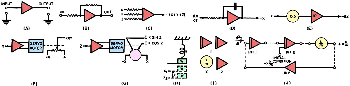
Fig. 2. Steps in setting up a problem for the analoque computer
to solve. See text for details on each individual operation.
The components of the computer have block diagrams that identify their functions
and serve as guideposts for the operator when he sets up a problem. See Fig. 2.
Fig. 2A is the symbol for an amplifier. Usually the amplifier is shown with
its input and feedback resistances (Fig. 2B). It is the ratio of the values
of these resistances that determines the gain of the amplifier.
Since all voltages are referred to ground, the ground terminals are usually not
shown. The basic amplifier can do many things, (a) It can add and when so doing
is called a "summing amplifier" or "summer," Fig. 2C. (b) It can perform integration,
Fig. 2D, and is called an "integrator." (c) With the aid of a potentiometer,
it can multiply by a constant (Fig. 2E). For this case the potentiometer is
adjusted so that it will divide any voltage such as x by 2. The amplifier is adjusted
for a gain of ten. (d) An amplifier in conjunction with a servo-controlled motor,
Fig. 2F, which drives the arm of a potentiometer can multiply or divide. (e)
For trigonometric functions, the amplifier (Fig. 2G) controls a servo-driven
sine-cosine potentiometer.
In each case, the amplifier is the heart of the computing element. Other devices
such as function generators for non-linear equations, limiters, relay amplifiers,
and recorders are used where required for a solution. The computer at Convair has
many combinations of these devices.
Now the visitor remarks, "These gadgets are all very fine. Let's see you solve
a problem with them."
That seems like a logical request so let us run through a simple problem to see
how the computer works.
Take a classical example, the spring supporting a weight. Fig. 2H. This
problem requires some set-up work before the computer can be of use. First we must
find an equation describing the problem. X1 is the position of W hanging
on the spring, k. X2 is the condition when W is displaced by some force
pulling the weight down. The equation expressing this system is m(d2x
/ dt2) = -kx where x is the displacement of the weight from its rest
position X1.
In order to set up the computer, the equation is rearranged to read: (d2x
/ dt2) = - (k/m) (x). The desired answers to this equation are the displacement,
velocity, and acceleration of the weight, W, at any time after the weight is released.
The computing elements (Fig 2I) needed for a solution are: two integrating amplifiers
(1), a potentiometer set at the ratio k/m (2), and an inverting amplifier to change
the algebraic sign (3).
Now we are ready to patch up the problem on the computer patchboard, Fig. 2J.
Assume, to start, that you have a voltage equal to d2x/dt2 on one end of a patch
cord. This is plugged to the input of Integrator 1. The output of this integrator
will be -dx/dt. This value is patched to Integrator 2 whose output will be x. Going
back to the equation, we note that d2x / dt2 = (k/m) (x) so
we patch the output of Integrator 2 to a potentiometer set at the ratio of k/m.
We still have to change the sign so the potentiometer is then patched to the
input of an inverting amplifier which changes the sign. At the output of the inverter
appears -(k/m) (x), which is equal to d2x / dt2 which is the
value we assumed to be the input to Integrator 1 in the first place. So, we patch
the output of the inverter to this point.
We now have taken care of everything but setting the system into operation. This
requires that we duplicate in the computer the initial conditions, i.e., the weight
is motionless because it has not been set into motion by releasing the force holding
the weight in the position where the displacement is -x (the sign is negative because
the force is in a downward direction). To put this initial condition into the computer,
a charge corresponding to the initial output voltage, -x, must be placed on the
feedback condenser of Integrator 2. There is no initial condition required at Integrator
1 because the output of Integrator 1, which is the velocity, dx/dt, at the start
of the problem, is zero.
The control switch of the computer, which is in the "Reset" position, is thrown
to "Operate" which is analogous to releasing the weight. The output voltage of Integrator
2 will rise and fall just as the weight rises and falls.
These three answers can be obtained on a recorder or other measuring device:
The displacement of the weight, x; the velocity of the weight, dx/dt; and the acceleration
d2x / dt2, Fig.2J.
This problem is a very simple one to solve either by "longhand" or with the computer.
The value of the computer can be appreciated if any of the parameters of the system
are varied. The answers appear instantly. Thus, it is possible to run a system from
"one end to the other" and be able to determine its capabilities at once.
Because of the comparatively lengthy set-up time on the patchboards, the Convair
computer has removable patchboards. This allows the operating station to be occupied
only during actual computation. While one operator is setting up a problem, another
can be using the machine. Fig. 1 shows the removable patchboard with a problem
patched in. It also shows portions of two operating stations. At either side are
the controls for each station. Answers may be read on the eight-channel recorders
in front as well as on the meter on the control panel. Trunk lines between stations
allow operators to "borrow" equipment appearing on adjacent patchboards.
The million-dollar computer is housed in a temperature- and humidity-controlled
area to insure minimum variations caused by temperature fluctuations or leakage
due to atmospheric moisture. Many factors were considered in the design and layout
of the computer: (1) High stability over long periods of time, (2) Isolation of
critical elements. (3) Modern, neat appearance. (4) Ease of operation and maintenance.
Needless to say, many problems had to be met and overcome in the design and construction
of the Convair computer facility. As various portions are placed into service, new
problems arise that require solutions and new techniques are developed. With the
completion of the computer facility, Convair will have a versatile, accurate, time-saving
device that is rapidly becoming an indispensable tool in the art of aircraft design
and manufacture.
Posted May 13, 2022
(updated from original post on 6/19/2015)
|