Map Your Fringe Area Signal Level |
||
Have you noticed how heavily burdened utility poles (formerly referred to as electric poles or telephone poles) are these days? Many of the decades−old creosoted wooden poles originally were designed to carry a single set of high voltage distribution lines (13.8 kV) and a multiconductor telephone cable containing twisted pairs. Look around now and you will see at least twice that number of cables, and often three times as many due to multiple coaxial and fiber optic cables and needing to route extra AC power circuits (of larger gauge to handle higher current) in increasingly crowded areas. Notice how many are leaning over (particularly at corners) and/or are being supported with additional guy cables and/or splints. Half a century ago when music, talk, and television was broadcast over the air, the need to string wire all over the landscape was not necessary. Some people complained about "ugly" TV and radio station broadcast antennas, but their numbers paled compared to all the cellular network towers littering the landscape these days, and the "carbon footprint" was way smaller. The "wireless revolution" is anything but wireless, and it certainly is not eco−friendly. Another article in this issue entitled "Television Signal Strength Calculation Charts" is useful here. Map Your Fringe Area Signal Level
Practical information on measuring and plotting signal levels to facilitate TV installation work. In a fringe or near-fringe area service organization, it is important for both the sales and service departments to know the signal level distribution (for each channel) throughout the district. Such information is of help in choosing a suitable receiver, deciding whether or not a booster is necessary, and selecting the correct antenna type for the location. There has been a definite need for a practical and useful link between propagated signal levels, service type field strength meters, and receiver performance. The signal level "Data-Print" on the facing page, together with the measuring equipment and measurement standards here introduced, represent a practical plan for predicting and solving signal level problems in a given locality. The charts can be used to predict local channel signal levels as a function of distance. Antenna gain and height can be linked directly to the chart information, thus assuming a more understandable significance. The method of making such measurements is simple and permits the service organization to take sample measurements in its own locality. The information thus obtained can be added to the "Data-Print" charts to give more specific data concerning stations in its own area. The "Data-Print" will then reflect the signal level variations due to terrain differences, climatic conditions, etc. Using the charts, range maps can then be prepared showing the location of specific signal level contours for each station. Finally, a sectionalized map of a single community or district can be prepared with finely calibrated contours and terrain height corrections. Such a map will enable a service organization to select the proper antenna and a booster, if necessary, for any installation without further measurement.
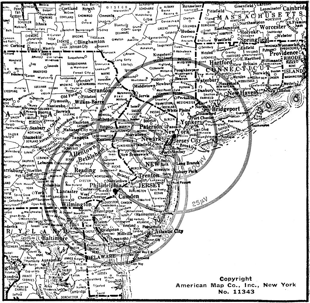
Fig. 1 - Signal range map for Channel 5 (N. Y.) and Channel 3 (Philadelphia). The receiving antenna for these measurements was a standard dipole, cut for each channel. For Channel 5, the 500 μv. radius is 60 miles from the transmitter: the 25 μv. radius is 104 miles. For Channel 3. the 500 μv. radius is 38 miles: the 25 μv. circle is the signal level 81 miles from the transmitter site. Copyright American Map Co., Inc., New York, No. 11343
Fig. 2 - A signal range chart for Channel 5 (N. Y.) and Channel 3 (Philadelphia) using a conical reflector receiving antenna to obtain the readings. Channel 5, whose transmitter is at the Empire State Building, delivers a 25 μv. signal over a radius of 112 miles and a 500 μv. signal at a radius of 64 1/2 miles. Channel 3 (which is transmitted from a suburban Philadelphia location) delivers a 25 μv. signal at a radius of 90 miles and a 500 μv. signal at a distance of 40 1/2 miles from the transmitter as shown by the concentric circles on the chart.
Fig. 3 - Signal range map for Channel 9 (N. Y.) and Channel 10 (Philadelphia). For Channel 9. the 500 μv. radius is 41 miles from the transmitter; the 25 μv. radius is 76 miles. The 50 μv. radius for Channel 10 was determined using dipole. conical reflector, and Yagi antennas. The circles show the effect of using succeedingly higher gain antennas. The yagi antenna will supply the receiver with a 50 μv. signal at 68 miles from the transmitter; the conical reflector at 62 miles; and the standard dipole will provide this figure at a distance of 49 miles. Field Strength Equipment The equipment used to take the field strength measurements for this article consisted of a field strength meter (the Transvision FSM-1A), a power converter, a "Variac," and a folded dipole, mounted on a thirty-foot mast, for each of the channels measured. The power converter was a Cornell-Dubilier Model 6R5 which converts 6 volts d.c. to 117 volts a.c. The power plug and cord were the type used with an auto trouble light so the 6 volts for the converter could be obtained by plugging into the cigar lighter receptacle of the car. The "Variac" was used to supply constant voltage to the field strength meter for each measurement. Thirty feet of 300-ohm twin-lead was used between the antenna and the meter. It was found advisable to keep the car engine running whenever measurements were taken to keep the car battery charged. Measurement sites must be chosen carefully. The antenna used for the measurements must be erected in the clear and away from large metallic objects, power lines, and telephone wires. In urban areas, lots, open fields, athletic fields, etc., are likely locations for taking readings and erecting the mast (use three ten-foot bolted or locked telescoping sections). Fringe area measurements can be conveniently made along the flat stretches of a turnpike and at various distances around the outskirts of small towns. Two ten-foot mast sections on a ten-foot rise or embankment will give the required thirty-foot elevation. It is important to realize that the more measurements made, the better the variables will average out. This permits construction of a smooth average curve of signal decline because of the many plot points. Signal Range Maps The signal decline charts on the "Data-Print" indicate the type of plot that can be constructed for any television area. Measurements were taken and charts plotted for Channels 3 (Philadelphia), 5 (New York), 9 (New York) and 10 (Philadelphia). The chart covers two channels in the low-frequency and two in the high-frequency television bands. For those channels not specifically covered, use the chart for the closest channel. For example, for the signal range of Channel 2, use the chart given for Channel 3; for Channel 7 use the Channel 9 chart, etc. The strength of the signal (in microvolts) can be obtained by taking a few sample measurements in your area and using the signal decline charts to predict signal levels at any given distance. For example, if the signal level obtained from your local Channel 5 station is only 500 microvolts at fifty-three miles instead of the 1000 microvolts (refer to Channel 5 signal decline chart), the entire microvolt scale is simply halved. The microvolt scale is changed by what-ever ratio exists between actual and chart readings for the range at which the sample measurement is made. The signal range maps are constructed from the information given in the signal decline charts. Each contour represents a certain signal strength for a particular station at a given distance from the transmitter location, as obtained from the chart for that station. The first signal range map (Fig. 1) depicts 500 and 25 microvolt contours for New York's Channel 5 and Philadelphia's Channel 3. These signal levels represent actual microvolts applied to the input of a receiver or to the 300-ohm input of a service type field intensity meter that has been calibrated accurately. It should be noted that similar microvolt contours for New York's Channel 5 and Philadelphia's Channel 3 are at different distances from the station. This is a result of different erp's, antenna heights, and terrain conditions. Thus, the factors of erp and transmitting antenna height have appreciable significance in the fringe range of a station. An explanation of the 500 and 25 microvolt choice is instructive. For the average television receiver manufactured during the last few years an input signal of 1000 microvolts (at the tuner input) was the level at which the receiver noise became apparent by very close observation of the line structure of the picture adjusted for normal contrast (first appearance of faint snow effect). When the signal level is at 50 microvolts, the snow effect is severe and the picture is near a point at which it cannot be considered tolerable for satisfactory viewing. With the new cascode low-noise type of tuner, levels of 500 and 25 microvolts are a better approximation. The maps show extended range possibilities of lower noise levels. It is true that these noise conditions vary from receiver to receiver and from channel to channel. Nevertheless, the values chosen represent an ultimate practical value. In summary, such maps will tell you, as a function of channel (low or high band) and erp of station, etc., the approximate microvolts of signal that can be expected at the receiver input at a given distance from the station. The logic behind the choice of a dipole reference is demonstrated in Fig. 2. Normally, gain figures of various commercial-type receiving antennas are given (or should be) with reference to the signal delivered by a standard dipole. For example, if an antenna with a gain of 6 db was used instead of a reference dipole in the case of New York's Channel 5, there would be twice as much voltage at the receiver input for each of the contour distances from the station. Likewise, readings taken from the microvolt scale on the signal level chart for Channel 5 on the "Data-Print" must be doubled. This indicates that the actual contour values of Fig. 1 are further separated from the station transmitters as a function of the gain of the antenna. This range extension factor is demonstrated in Fig. 2 for a conventional conical-reflector type of antenna with a gain of 3.5 db on Channel 5 and 2.5 db on Channel 3. Just how much farther the contours fall can be calculated from the signal level charts on the "Data-Print." Simply raise the curve by the db gain introduced by the antenna and read the microvolt-distance figures directly off the chart for the new curve. With these new figures, draw the new contour. The service organization can follow this same procedure for whatever type antenna used. For example, the 500 microvolt contour for Channel 3 is 38 miles out, using a standard dipole with the measurement standards specified. This point on the chart is at the -26 db level (chart 1). With a conical-reflector at this distance, the signal level at the receiver would be 1.33 times 500 or 665 microvolts (2.5 db antenna gain). The actual 500 microvolt level for the conical-reflector would be located at a distance represented by a signal decline of 28.5 db (26 pi us 2.5). On the chart, this level is located at the 40 1/2 mile point. The New York's Channel 9 portion of Fig. 3 shows the 500 and 25 microvolt points for this station. Notice that these contours are nearer to the station location than they were for the low-band stations although transmitting powers are higher. To demonstrate further the influence of antenna gain on microvolt contours, the Channel 10 (Philadelphia) portion of Fig. 3 shows the 50 microvolt contours for a dipole, a standard conical-reflector, and a Channel 10 yagi. Notice how the 50 microvolt contour can be extended further and further from the station with antenna gain. A number of important facts are revealed by the signal decline charts and range maps. The rate of signal decline is much faster than the practical rate at which gain can be added to an antenna system. For example, using the Channel 3 signal decline curve we note that the 1000 microvolt contour is at 31 1/2 miles . Just 26 miles beyond this, or at a range of 57 miles, an antenna with a phenomenal gain of 20 db would be needed to bring the signal up to the 1000 microvolt level. The signal decline averages one decibel per mile over most of the range. We cannot expect too much from antenna systems in fringe reception. For example, let us assume we have a good quality receiver that does not show any effect for a 500 microvolt signal. Now, at a range of· 70 miles (Channel 3) we have a signal of approximately 45 microvolts. This level produces a useful signal but one with high snow content. Suppose, in our enthusiasm, we decide to double the antenna height (up to 60 feet) and use a high-gain yagi (12 db). This more elaborate installation raises our signal by perhaps 15 db (assuming a conservative 3 db line, installation, and mismatch losses). This brings the signal level up to approximately 350 microvolts which is a decided improvement but still not high enough to take the snow effect out of the picture. This example also indicates why you should not expect too much from the increasing antenna height-it is quite a jump from a 30 footer to a 60 footer. The improvement is there and is worthwhile but don't expect miracles.
Posted October 18, 2021 |
||

 By Edward M. Noll and Matthew Mandl