April 1957 Radio & TV News
 [Table
of Contents] [Table
of Contents]
Wax nostalgic about and learn from the history of early
electronics. See articles from
Radio & Television News, published 1919-1959. All copyrights hereby
acknowledged.
|
Simpson Electric is a name most RF Cafe
visitors are probably familiar with as being the maker of high quality analog multimeters,
with the
Simpson 260 line being the most famous (it is still manufactured
today). Not as many people, however, know that Simpson also used to make oscilloscopes.
This article from a 1957 issue of Radio & TV News magazine was written
by a Simpson Electric engineer whose job was, in part, to respond to questions asked
by users. It covers basic operations like how to calibrate the display, adjust
 the horizontal time base and vertical amplitude
scales, and how to synchronize the display with the input signal. Some explanation
of how to interpret periodic and pulse type waveforms is provided as well as tips
on how to avoid overloading and possibly damaging the instrument. the horizontal time base and vertical amplitude
scales, and how to synchronize the display with the input signal. Some explanation
of how to interpret periodic and pulse type waveforms is provided as well as tips
on how to avoid overloading and possibly damaging the instrument.
Aficionados of vintage oscilloscopes might want to visit the
Oscilloscope Museum
website, and Simpson Electric fans can visit the Simpson260.com website for just
about any
Simpson user's manual.
Questions and Answers on Oscilloscopes
 By Robert G. Middleton By Robert G. Middleton
Chief Field Engineer, Simpson Electric Company
Replies to the queries the manufacturer most often gets from technicians on this
important instrument.
Of the many questions manufacturers of oscilloscopes are asked, the most common
is, "Which is the right pattern? I can get nearly any pattern I want on the scope
screen." The question is too complex to be answered simply. What is involved here
is a basic understanding of the operation and application of the instrument. The
"right" pattern, of course, is obtained only when operation and application are
correct. Still, the high degree of frequency with which the question is asked, even
in this era, justifies a fundamental review of the instrument and the nature of
the phenomena which it is used to examine.
Basic Scope Display
The display of a 60-cycle sine-wave signal is very basic, and an instructive
point from which to start. Turn on the scope and adjust the intensity and focus
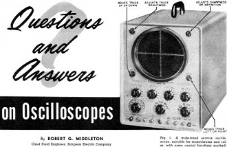
controls to obtain a bright and well-focused horizontal trace (see Fig. 1).
The vertical and horizontal centering controls are adjusted, as required, to center
the trace on the scope screen.
If the vertical-gain controls of the scope are advanced to maximum, a pattern
is obtained on the scope screen even though there is no signal input to the scope.
This is a very puzzling point to the beginner, and is explained as follows: the
scope input system has a very high impedance. For this reason, the exposed input
terminals pick up stray 60-cycle fields about the bench, producing substantial vertical
deflection. Note that, when a 1-megohm resistor is shunted across the scope input
terminals, the pick-up is eliminated. This is the reason that stray fields do not
enter the scope in normal circuit testing - the circuit impedance shunts the scope
input, so that any stray pick-up is not observable.
To display the 60-cycle pattern in proper form, the coarse frequency control
is set to a position which includes 60 cycles. For the scope illustrated in Fig. 1,
the control would be set to the 14- to 250-cycle position. The fine-frequency control
is then adjusted to obtain one, two, or more cycles, as desired, of pattern.
To lock the pattern on the screen, so that it does not "run" horizontally, the
function switch should be set to a suitable sync position, such as line-sync in
the case of this 60-cycle wave, and the sync-amplitude control is advanced just
sufficiently to lock the pattern tightly. This 60-cycle sine-wave pattern may appear
very elementary, but it has some important properties which are worthy of note.
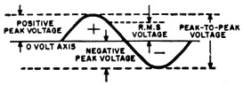
Fig. 2 - A sine wave is used to illustrate various ways
to measure voltage.
Fig. 2 shows such a sine-wave pattern, with the important" values depicted.
The average value of the symmetrical sine wave is zero, and falls along the zero-volt
axis, or resting position of the trace when no input signal is present. The total
excursion of the waveform is a measure of its peak-to-peak voltage. The peak-to-peak
voltage is made up of a positive-peak voltage and a negative-peak voltage, as shown
in Fig. 2. The r.m.s. voltage is equal to 0.707 of the peak value; this r.m.s.
voltage is the value which is indicated by an a.c. service voltmeter.
Why these three values? The first a.c. voltage value which was recognized was
the r.m.s. value. This has its origin in power work, and is still used in the measurement
of line voltage, transformer voltages, and heater voltages. Power work started out
with d.c. power sources (even in some areas today, power lines still supply d.c.
voltage). When a.c. power became common, it was desired to measure a.c. voltage
in units such that the amount of light, or heat, or power obtained from a 117-volt
a.c. line would be the same as that obtained from a 117-volt d.c. line. Thus if
a 117-volt (r.m.s.) a.c. line is connected to a soldering iron, just as much heat
will be obtained as if a 117-volt d.c. line is connected to that iron.
However, the advent of TV brought in a new requirement: vacuum tubes in most
cases respond upon the basis of the applied peak-to-peak signal voltage. In some
cases, the tube responds to the positive-peak or to the negative-peak voltage which
is applied - this depends upon operating bias. In any case, these newer units of
voltage are of chief significance in servicing electronic circuits. The peak voltage
of a sine wave is equal to 1.414 times its r.m.s. value, and the peak-to-peak voltage
of a sine wave is equal to 2.83 times its r.m.s. value. It is evident that the peak-to-peak
voltage of a sine wave is double the value of either the positive-peak or of the
negative-peak voltage. This is so only because a sine wave is symmetrical.
Pulse Voltages
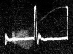
Fig. 3 - This asymmetrical pulse waveform is more typical
of those encountered in TV than the sine wave. Note the unequal positive and negative
peaks.
Most television waveforms are not symmetrical. A simple pulse waveform like the
one shown in Fig. 3 has a positive-peak voltage which is unequal to its negative-peak
voltage as shown in Fig. 4. The peak-to-peak voltage of the pulse is equal
to the sum of its positive-peak voltage plus its negative-peak voltage.
It should be noted that the average value of a pulse waveform - as of all complex
waveforms - is zero. This average level falls along the zero-volt level on the screen;
that is, it falls along the resting position of the beam when no input signal is
applied to the scope. It is this basic property which is utilized in measuring the
positive- and negative-peak voltages of the waveform. Note that, in any pulse or
complex waveform, the area of the pattern above the zero-volt axis is exactly equal
to the area of the pattern below the zero-volt axis. This is a necessary consequence
of the fact that the average value of the waveform is zero.
When a pulse waveform is applied to the input of a d.c. voltmeter, the pointer
indicates zero volts. Again, this observation is the result of the fact the average
value of the waveform is zero. However, when the pulse voltage is applied to the
input of an a.c. voltmeter, the indication obtained depends upon several factors.
In general, the indication will be largely meaningless. The pulse waveform does
have an r.m.s. value, but this is somewhat difficult to determine, and is of little
interest to the service technician. The indication obtained will depend upon the
frequency characteristics of the test instrument, which way the test leads are applied
to the pulse source, and other factors. Of course, some voltmeters have a peak-indication
function, or a peak-to-peak indication function. In such case, a useful measurement
can be obtained unless the pulse repetition rate is low and the pulse is narrow.
Because of these various considerations and reservations, the use of the techniques
that do not involve the scope for waveform examination can be seen to have serious
shortcomings.
Voltage Measurements
If the oscilloscope is to be the instrument for reliably measuring waveforms,
as well as observing them for appearance, how can dependable measurements be made
on an instrument with which, by adjustment, we "can get any pattern we want?" Indeed,
these questions pertaining to measurement, and especially to the measurement of
peak-to-peak value, fall into the most-frequently-asked category.
Most scopes nowadays provide a source of calibrating voltage for reference. The
scope shown in Fig. 1, for example, makes an 18-volt peak-to-peak sine-wave
voltage available through a binding post on the front panel. (Where a calibrating
standard of this kind is not built in, a sine wave of known amplitude may be introduced
externally with no change in the remainder of the measurement procedure.) When a
lead is connected from this binding post, or other source, to the vertical-input
terminal of the scope, a known voltage of 18 peak-to-peak volts develops a sine-wave
pattern on the screen.
If the vertical-gain controls are adjusted to make the sine wave occupy a total
height of 18 squares on the calibrated grid or screen, each square will evidently
measure one peak-to-peak volt. Now the calibrating lead can be disconnected and,
provided that the vertical-gain controls are left untouched, another signal voltage
can be measured. After this unknown signal is applied, a count is made of the squares
of vertical deflection it achieves. This is its peak-to-peak voltage.

Fig. 4 - Positive and negative peak amplitudes are unequal
for the pulse, but areas enclosed by each peak are equal.
Of course, signal voltages subject to measurement vary widely in amplitude. Some
may be so large that they will drive the beam off-screen when applied to the scope
with the same vertical-input settings used for the reference voltage; on the other
hand, some of these voltages may be so small as to fail to produce measurable deflection.
To meet this situation, a step attenuator, or coarse vertical-gain control is provided.
Generally this step attenuator is arranged in decimal steps, which are most convenient.
The continuous, fine vertical-gain control, or the vertical vernier, is still
left untouched, but the coarse control is turned in either direction the number
of steps required to obtain a satisfactory deflection on the screen for the voltage
being measured. If the coarse attenuator has been turned up one step to increase
the sensitivity of the scope by ten times as compared to its former position, then
each vertical square will represent .1 peak-to-peak volt, instead of 1 volt. On
the other hand, if the attenuator has been turned down one step, to reduce an oversize
waveform, each square will now represent 10 peak-to-peak volts. If the attenuator
has been turned down two steps, each square will represent 100 peak-to-peak volts.
Thus the utility of a decimal step attenuator lies in the fact that the basic
calibration of the scope is unchanged - only a decimal point is shifted. Some scopes
may have a step attenuator that changes sensitivity by some factor other than 10.
These can be just as accurate, but they are not quite as convenient, as they may
involve a small amount of arithmetic.
While a relatively simple pulsed waveform has been chosen to illustrate the technique
of measurement involved, the procedure is used unchanged with the most complex wave-shapes.
In fact, most technicians prefer, while taking peak-to-peak measurements, to reduce
the horizontal gain or width control to zero. This reduces all waveforms, no matter
how different or confusing in shape, to a common denominator - a single vertical
line. Since the length of that line is the true peak-to-peak value, irrespective
of shape, measurement procedure is simplified.
Avoid Overload
Another question which is often asked concerns distortion of the displayed waveform
which results from application of excessive signal voltage to the scope input. It
must be recognized that it is quite possible to overdrive a scope amplifier, just
as may be done with any other amplifier. When overload occurs, the waveform is clipped
on the top, or bottom, or both. The resulting distorted pattern can be very misleading.
To avoid scope overload, a simple operating rule should be followed at all times:
Adjust the vertical-input controls so that the continuous attenuator is operating
on the upper portion of its range. If necessary, the coarse attenuator can always
be advanced a step or two, to permit this condition. The reason for this precaution
is that the output from the coarse attenuator is generally applied to the grid of
the scope input stage, while the continuous attenuator works in the cathode circuit.
It is grid overdrive which provides overload and clipping.
Posted June 23, 2022
(updated from original post on
11/8/2013)
|