|
|||||||||||||
 |
|||||||||||||
Electronic Measurements Using Statistical Techniques
|
|||||||||||||
I learned (or, "leared," in MN Somali daycare lingo) a new word today - ergodic - from a 1968 issue of Electronics World magazine. Ergodicity is a concept from mathematics and physics describing systems where the time average of a property equals its average across all possible states (space average). In simpler terms, a system is ergodic if, over time, it explores all possible states in a way that reflects the overall statistical distribution of those states. In physics and dynamical systems: An ergodic system eventually visits all parts of its phase space uniformly. For example, in statistical mechanics, the ergodic hypothesis suggests that a physical system will, over time, spend time in each state proportional to its probability, allowing macroscopic properties (like temperature or pressure) to be derived from time averages. In probability and stochastic processes: A process is ergodic if its statistical properties (like mean or variance) can be deduced from a single, sufficiently long sample path. For instance, a fair coin flip sequence is ergodic because the long-term proportion of heads will converge to 50%, matching the theoretical probability. Electronic Measurements Using Statistical Techniques
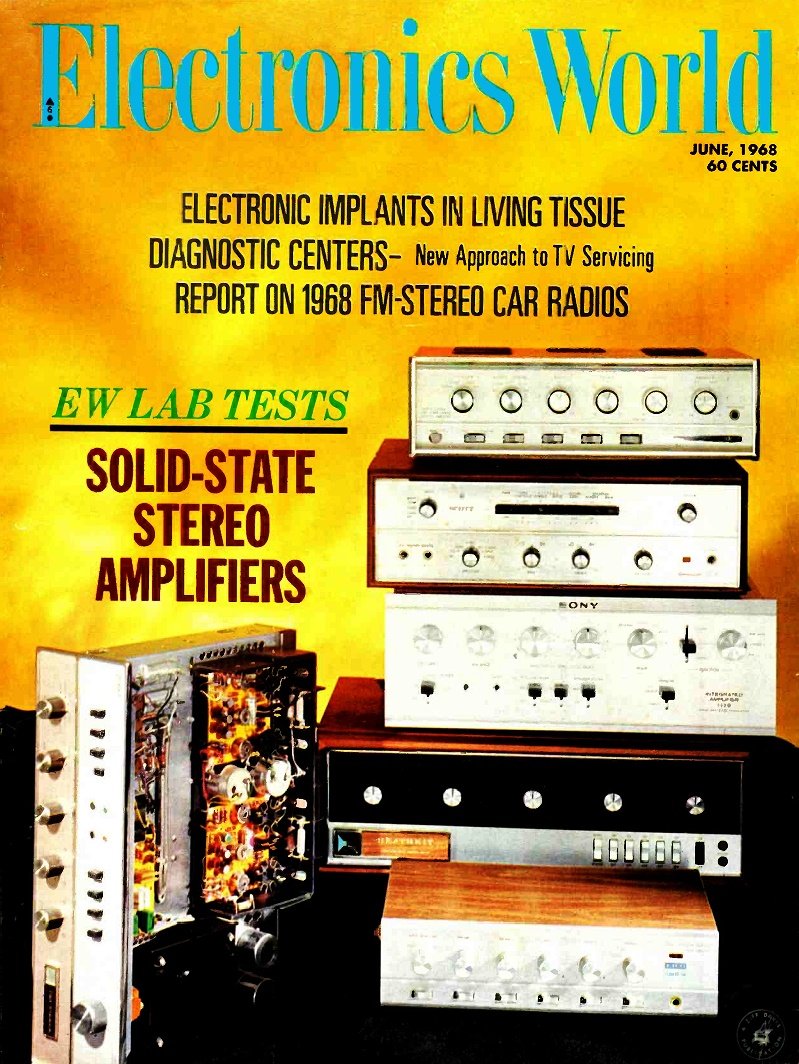
Fig. 1 - Volts-time history of random data from four noise generators. By Sidney L. Silver Many physical phenomena produce nonperiodic, random signals that must be analyzed by a statistical study of their average characteristics. Examples include thermal and shot noise, static interference, irregular mechanical stresses, or vibration. Techniques used are probability density, distribution correlation, spectral analysis. In many branches of applied science and engineering, there occur problems involving the measurement of physical quantities whose solution depends upon the proper interpretation of the relative amplitude, phase, and frequency characteristics of complex waveforms. Harmonic functions, for example, produce data which may be separated into simple periodic waveshapes in order to determine the various frequency components and their energy distribution. Such quantities are said to be "deterministic" since their instantaneous values can easily be predicted as a function of time. In practice, however, many physical phenomena produce non-periodic or random information, which can best be defined in statistical terms. These quantities are described as "probabilistic" since their instantaneous amplitudes cannot be predicted with complete certainty at any future period of time. Instead, they must be analyzed by making a statistical study of their average characteristics over a specific time interval. Typical examples of measurable quantities which produce random data are temperature fluctuations in an industrial control process, noise and vibration from high-power jet and rocket engines, buffeting forces on an aircraft at gust wind velocities, acoustic pressures generated by turbulent air, notion of a structure caused by seismic excitation, stresses of a stabilized ship exposed to rough ocean waves, static interference in communications systems due to atmospheric disturbances, shot noise in a vacuum tube, and thermal noise in a resistor.
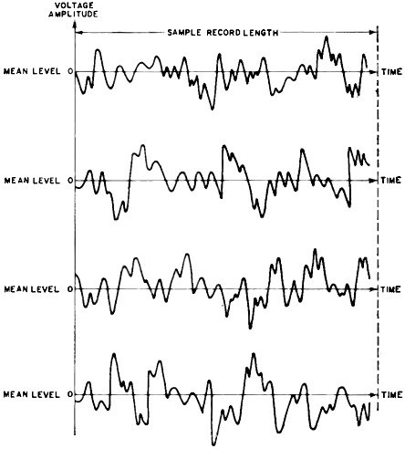
Fig. 2 - A graphic determination of probability density function.
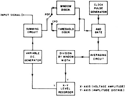
Fig. 3 - Amplitude distribution analyzer measures the probability density and cumulative probability distribution.
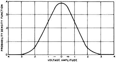
Fig. 4 - A normal probability density function curve.
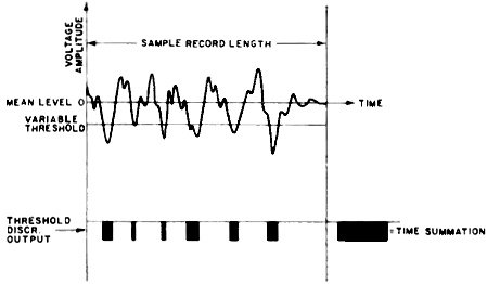
Fig. 5 - Evaluation of cumulative probability distribution.
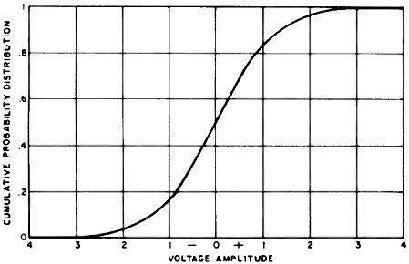
Fig. 6 - Cumulative probability distribution function curve.
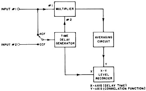
Fig. 7 - Correlation analyzer is used to measure autocorrelation and the cross-correlation functions as described in text.
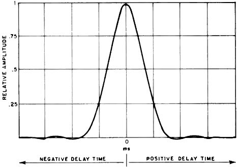
Fig. 8 - Autocorrelation function of wide -band random noise.
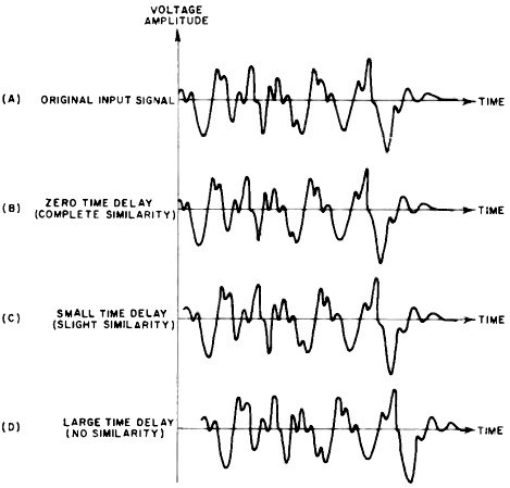
Fig. 9 - Time-shifting of the sample record during autocorrelation scanning process to assess degree of similarity.
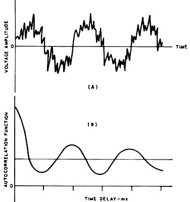
Fig. 10 - (A) Voltage-time plot of sine wave immersed in noise. (B) Resulting autocorrelogram extracts the periodic component.
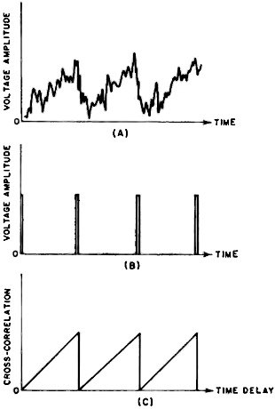
Fig. 11 - (A) Time plot of sawtooth wave in noise. (B) Time function of reference pulses. (C) Cross-correlogram.
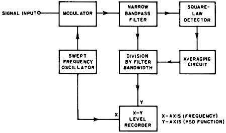
Fig. 12 - Functional diagram for power spectral density analyzer.
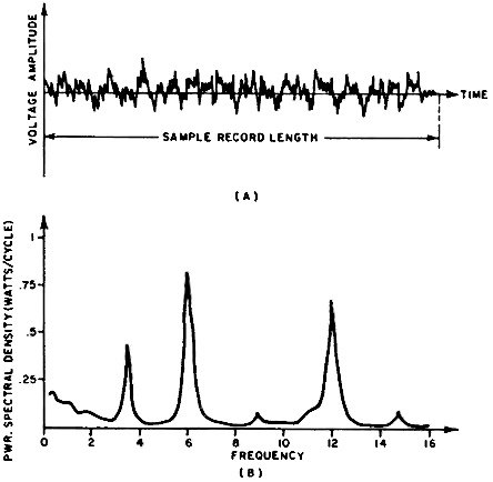
Fig. 13 - (A) Voltage-time plot of random variations. (B) Power spectral density curve shows relative power distribution vs frequency. Characteristics of Random\Waveforms To demonstrate the nature of a random process, the voltage-time history of a number of random -noise generators of identical design and construction is plotted on a chart recorder (Fig. 1). For convenience, the mean value of each waveform is arbitrarily chosen to be zero. By operating all generators simultaneously the collection, or ensemble, of sample records is observed to fluctuate erratically, each waveform representing only one of many possible occurrences. Clearly each observation of the instantaneous magnitudes is a unique phenomenon, since the waveshapes never exactly recur in a finite time period. Any attempt to make a precise, detailed analysis of the fluctuations by observing previous values would be meaningless. Theoretically a thoroughly accurate implementation of the random process would involve an infinite number of sample records over an infinite time period. In practice, however, only a finite number of noise generators need be considered, since the long-term average characteristics of the amplitude values remain unchanged by any additional noise sources. By applying statistical concepts to the measurement of these random signals, it is possible to quantitatively describe them by computing the integrated values of the waveforms over a predetermined interval of time. Some of the apparent statistical variations can then be determined and a reasonably accurate estimate of the future values easily obtained. If the statistical properties of an ensemble (of sufficient length) do not vary with time, the ensemble is said to be stationary. This implies that the mean value, the amplitude distribution about the mean value, the number of peaks per unit time, and the predominant frequencies, if any, of the collection of sample records is the same. In this article, reference will be made only to those stationary random phenomena with ergodic properties, i.e., where the time average of a single sample record is equal to the corresponding ensemble average value, thus leading to the same statistical results. Fortunately, most statistical phenomena are generally ergodic so that such random data can be properly measured from a single sample record. In the electronic measurement of random information, there are three domains in which the statistical parameters may be processed: amplitude domain (probability density and distribution), time domain (correlation), and frequency domain (spectral analysis). Any of these can be implemented through analog or digital techniques. Amplitude Domain Measurement An important means of characterizing random data in the amplitude domain is the probability density function (PDF), which describes the probability that the waveform amplitude will assume a value within some specified range of values at any interval of time. Initially, the quantity to be analyzed is picked up by a suitable transducer which converts the original signal into electrical form. The computation of the PDF is most conveniently accomplished by recording a sample of the signal on a magnetic tape loop. During the playback mode, the signal is continuously compared with a reference level, or "window," discriminator which "slices" the sample record into a very narrow amplitude range (Fig. 2), thus allowing only that portion of the signal to pass through the system. The signal waveform is then integrated over the time the signal spends within the amplitude window. At the end of each tape revolution, the integrated signal is plotted and the window voltage is moved one incremental step before the next integration cycle begins. This process continues until the scanning band sweeps the entire amplitude range of the input signal, producing a graphic representation of the amplitude distribution curve. A functional block diagram of a typical amplitude distribution analyzer is shown in Fig. 3. In the PDF mode of operation, the input signal is nixed with a variable d.c. potential. This provides a bias voltage which allows different levels of the waveform to be sampled by the window discriminator, and simultaneously shifts the X-axis of the graphic recorder. Each time the instantaneous value of the signal falls within the limits of the window, the and gate opens and passes 1 MHz clock pulses to the averaging circuit. By this means, a measure of the total number of pulses passed by the window circuit is obtained, expressed is a percentage of the total number of pulses generated. The time average may be obtained either by a true integrator (consisting of an operational amplifier with feedback capacitor), or by a low-pass RC filter which continuously smoothes the amplitude fluctuations. In general, true averaging is employed when the scanning process is accomplished in discrete steps (stepped scan), and RC averaging employed when a continuous scan sweeps the window. Finally, the required division of the average sampling time by the window width (fixed amplitude window voltage) yields the probability density function. Applying this parameter to the Y-axis of the level recorder produces a plot of PDF vs. voltage amplitude. Fig. 4 shows a normal, Or "Gaussian," PDF curve which is frequently encountered in random data measurement. Here the higher portions of the symmetrical curve correspond to the region where most of the input signal values occur, while the lower sections indicate values which rarely occur. The area of the curve is based on a scale of unity (or 100 %), so that any given area under the curve may be expressed in terms of a percentage of all values represented by the entire cure. Thus, for example, the probability that the instantaneous amplitude values of the input lie within a range bounded by zero and +3 volts, is 50. An alternate method of evaluating the amplitude distribution of a random waveform is a measure of the "cumulative probability distribution" (CPD), which contains the same information as the density function but presents it in a different form. The value of the CPD function is defined as the probability that the input signal is equal to, or below, a given amplitude. In this mode of operation, one of the two thresholds of the window discriminator shown in Fig. 3 is eliminated, thus extending the amplitude slice to include all of the magnitudes that are less than, or equal to, the remaining threshold. Initially, the reference level is set below the maximum negative value of the sample record to be examined. As the threshold voltage sweeps upward from negative to positive values (Fig. 5), an increasing portion of the input signal will lie below the reference level. By com- paring the proportion of time that the signal falls below the threshold to the total sampling time, a plot of the CPD function vs voltage amplitude is automatically produced (Fig. 6). At the completion of the scanning process, the entire signal waveform lies below the reference level and the integrated output is considered to be 100%. The principal applications for amplitude distribution measurements include the determination of threshold levels in mechanical stress analysis, detection of non-linear structural characteristics, surface and thickness instrumentation, and testing for normality of random data. The Domain Measurement One of the most powerful techniques used to describe the properties of random fluctuations in the time domain is the correlation function. The correlation concept determines the extent to which a future value of a random quantity will be the same as preset value of that quantity. By establishing a measure of similarity between two waveforms, or by determining the influence of one signal upon another, a quantitative analysis of the degree of randomness may be obtained. An important parameter employed in the computation of random data is the "autocorrelation function" (ACF) . This quantity refers to the dependency of a random signal upon a time-shifted version of itself, and provides a convenient means of determining the presence of a periodic signal obscured in a background of random noise. To implement this process, it is necessary to delay the random signal by a variable time displacement, multiply the signal value at any instant by the value preceding the delay time, and finally average the instantaneous product value over the total time of the sample record. Fig. 7 shows a typical ACF analyzer which operates in conjunction with a special-purpose instrumentation tape recorder. In this arrangement, a time sample of the signal to be analyzed is recorded on a magnetic tape loop, and fed to a time-delay generator to provide the necessary lag time. The variable time displacement is obtained by means of a movable playback head which automatically advances one small step for each revolution of the tape loop. Both the input and the output of the delay generator are then multiplied and time-averaged so that at the end of each integration cycle, the output appears as a series of discrete plots on the curve. hi some instruments, correlation values are measured while the delay time is continuously varied through the time displacement of interest, so that a continuous output curve is obtained. The sample record is recirculated until the information at each time delay is completely scanned and a graph of ACF vs time displacement is plotted on the X-Y recorder. Fig. 8 shows an ACF plot, called an "autocorrelogram ", which is typical of wide-band random noise. Assuming that the curve is plotted on positive and negative delay values, the graph is observed to be a sharply peaked symmetrical pulse which reaches a maximum value at zero time delay. The pulse then diminished to very low values until the correlation function reaches zero at large time delays. In order to interpret the form of the ACF curve, the relationship among the time-displaced versions of the input waveform is given in Fig. 9. At zero delay time, the random fluctuations applied to each input of the multiplier are in-phase. Since each positive and negative ordinate in (A) is identical to its counterpart in (13), the product of both values contributes a positive term to the sum. As the delay time increases during the scanning process, the waveform becomes less and less related to itself in (C), until the point is reached in (D) where the similarity is completely destroyed. Now that each positive product value is offset by another negative product, the sums rapidly decrease and the ACF reading falls effectively to zero. If a sine wave were fed to the ACF analyzer, the autocorrelogram would also be sinusoidal, having the same frequency and harmonic content as the input signal but dropping all phase information. It is reasonable to expect, therefore, that an ACF measurement of a wide-band noise record containing a hidden sine-wave component (Fig. 10A) would have some of the characteristics of both the random noise and the periodic signal. The resulting autocorrelogram in Fig. 10B indicates the peaked curve at zero delay, with the sinusoidal component persisting over all time displacements. Clearly the correlation technique makes it possible to detect and recover periodic information by greatly improving the signal-to-noise ratio (as much as 40 dB) of an incoming signal. Now that the frequency of the periodic signal to be extracted from the random noise is known, a more powerful technique, called the "cross -correlation function" (CCF), may be applied. This is accomplished by switching the ACF analyzer, shown in Fig. 7, to the CCF mode of operation. In this arrangement, the random signal fed to the direct input of multiplier #1 is independent of an external periodic waveform applied to the time-delay generator. Since the delayed input to the instrument is now a pure sine wave of the same frequency as the hidden periodic signal, the CCF analyzer produces a still greater improvement in signal-to-noise ratio and, in the ideal case, reduces the noise components of the signal to zero. An important advantage of this method over autocorrelation is that phase information is preserved, so that the resultant cross-correlogram is a proportional reproduction of the original time function. Another method of detecting a signal masked by extraneous noise is indicated in Fig. 11. This technique consists of cross-correlating the obscured signal (Fig. 11A) with a series of narrow pulses (Fig. 11B) which have the same fundamental frequency as the obscured signal. The resultant CCF curve (Fig. 11C) reveals the hidden signal to be a triangular wave. The cross-correlation technique may be employed to establish a possible "cause and effect" relationship between a disturbing sound source and a reverberant condition. In acoustic vibration problems, for example, cross-correlation is useful in determining the transmission paths and propagation velocities of a random vibration source. By placing one microphone close to the source of the disturbance and moving another microphone to different locations in sequence, a CCF computation is performanced for each point. If multiple sound paths exist the cross-correlogram will contain one peak for each sound path, while unrelated disturbances will rapidly correlate to zero. The delay value at each peak corresponds to the transmit time of the transmission path, and the ordinate of each peak indicates the relative contribution of each sound source. Frequency Domain Measurement Since random waveforms are characterized by the relative distribution of their frequency content, the analysis of non-periodic signals may be obtained in terms of the "power spectral density" (PSD) function. This parameter describes the harmonic composition of random data in terms of the mean square, or average power distribution over the frequency spectrum. To make an analysis, it is necessary to filter the input signal and average the squared instantaneous value over the total sampling time. In the PSD analyzer shown in Fig. 12, the data stored on a magnetic tape loop is heterodyned in the modulator by the output of a swept local oscillator. The modulator output is then fed to a highly sensitive narrow bandpass filter (with a fixed center frequency), which extracts that portion of the signal whose frequency range lies within its passband. The frequency components are detected by the squaring circuit and averaged by an RC filter whose time constant is set equal to the sample record length. Where a true integrator is used for averaging, the transient produced by the tape splice is used to derive a trigger pulse in order to reset the integrator at the end of each tape loop period. The required division of the mean square value of the averaging network by the filter bandwidth may be obtained by a proper scale calibration. As the sweeping oscillator scans the frequency range of interest, the center frequency of the bandpass filter is progressively moved, and output of the analyzer is displayed as a continuous plot of PSD function vs. frequency. In Fig. 13A, a sample voltage-time history record is shown of an undesirable random vibration, such as that produced by industrial machinery. By feeding this data into the PSD analyzer, the resultant power spectral density curve (Fig. 13B) shows how each peak level represents the signal contribution within the sample bandwidth. Since the total power distribution is equal to the entire area under the curve, the power in each of the peaks can be calculated from their individual areas. Now that the hidden components in the frequency domain are easily identified, and knowing the rotational speed of the machine parts, the disturbing vibration source can be located and eliminated. Where the phenomena being investigated involve the analysis of two related random processes, some knowledge of the phase relationship between the two quantities is sometimes required. For example it may be necessary to determine to what degree an acoustic source of vibration is responsible for the mechanical vibration in a metallic structure. This can be accomplished by means of a "cross-spectral density" (CSD) analyzer which measures the linear relationship between the power spectral density data represented by the two sample records. The statistical concepts discussed have been restricted to the analog measurement of stationary random data. Since the processing techniques do not, for the most part, apply to the analysis of non-stationary random waveforms (whose statistical properties change with time), more sophisticated methods must be developed to handle such data. |
|||||||||||||
 |
|||||||||||||
|
|||||||||||||

|
||||||||||||||||||||||||||||||||||||