|
June 1957 Radio-Electronics
 [Table of Contents] [Table of Contents]
Wax nostalgic about and learn from the history of early electronics.
See articles from Radio-Electronics,
published 1930-1988. All copyrights hereby acknowledged.
|
This "Harmonic Analysis Made
Easy" article from a 1957 issue of Radio-Electronics magazine presents
a brilliantly clever graphical method for performing harmonic analysis without complex
mathematics or the aid of a computer. By breaking down a waveform into discrete
ordinates every 30 degrees, the technique transforms Fourier analysis into a manageable
visual process, and skipping the messy math. Author Arthur Shulman's approach is
particularly ingenious in how it handles vector addition: plotting each ordinate's
value at its corresponding phase angle on a vector diagram automatically accounts
for trigonometric multiplication. The resultant vector's length and direction directly
reveal the harmonic's amplitude and phase. This method makes visualization remarkably
simple even without computational aid. By constructing vector polygons, engineers
could approximate a square wave using its fundamental and third harmonic components
(although a true square ware contains an
infinite number of odd
harmonics),
achieving practical accuracy for most applications. The graphical representation
turns abstract mathematical concepts into tangible geometric operations, allowing
the decomposition of complex waveforms using only drafting tools.
Harmonic Analysis Made Easy - Analyze harmonics without
higher mathematics
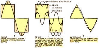
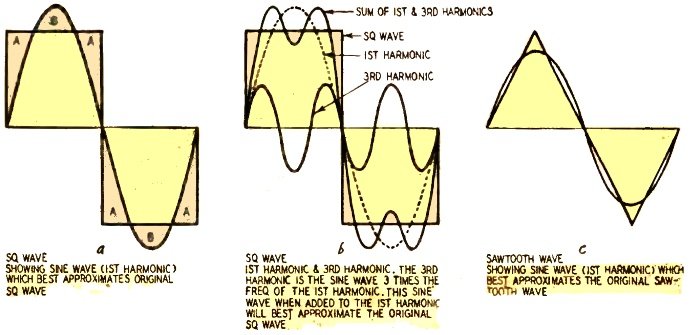
Fig. 1- Waveforms and their sine-wave approximates.
By Arnold R. Shulman
Most of us, while watching a waveform on an oscilloscope, have wished we could
measure the harmonic content. Many of us know that the harmonic content of any wave
can be determined by Fourier analysis. The trouble is that Fourier analysis requires
a knowledge of higher mathematics. Fortunately there is a method for determining
the harmonic content of a wave without using higher mathematics.
Sine waves have been adopted in engineering as the fundamental waveform. Sinusoidal
voltage is the only voltage waveform such that, when applied to a resistance, inductance
or capacitance, the current will have the same waveform. By using the sine wave
as a reference, a waveform can be analyzed into a number of sine waves of different
frequencies. This is Fourier analysis.
These sine waves of different frequencies are called the first harmonic or fundamental,
second harmonic, third harmonic, etc.

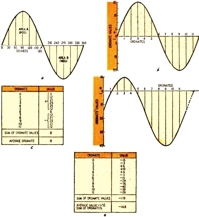
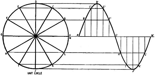
Fig. 2 - Sine waves with their ordinates and ordinate values
charted.
Fig. 1-a shows a square wave. It doesn't look anything like a sine wave,
but the figure shows that a sine wave can be drawn to approximate it. The sine wave
that will best approximate this square wave will have a definite phase and magnitude
with respect to it. This best-fitting sine wave is the first harmonic. If the square
wave is to be applied to a circuit, its effects may be calculated by assuming that
the first-harmonic sine wave was applied and by doing the calculations based on
that waveform.
Practically all formulas used in electrical engineering are based on sine waves.
Most instruments are calibrated for them - a square wave would cause the average
multimeter to read 11% high. The ability to approximate any wave with sine waves
is extremely important.
Actually the first harmonic is a poor approximation of the square wave. The shaded
areas A are not included, and area B is outside the square wave. The next step is
to find a sine wave of another frequency which, when added to the first harmonic,
will more closely approximate the square wave, adding to the areas marked A and
subtracting from the areas marked B. The third harmonic (a sine wave three times
the frequency of the first harmonic) will do that (see Fig. 1-b). If appropriate
higher harmonics were found and added to the first and third, a closer approximation
would be found.
It is evident that the first harmonic is a good approximation of the saw-tooth
wave in Fig. 1-c. It could be used in many calculations without introducing
a significant error. However, Fourier analysis permits any continually periodic
waveform to be represented and measured.
Graphic Analysis
The graphical procedure which follows is a close approximation to the accurate
mathematical solution (see equation at the head of this article). It is particularly
important because in most practical situations it is necessary to find only a few
harmonics. The higher-frequency components are usually so small that they have little
effect.
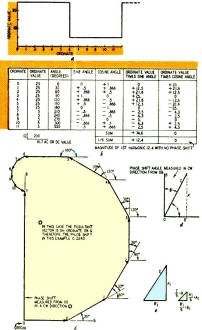
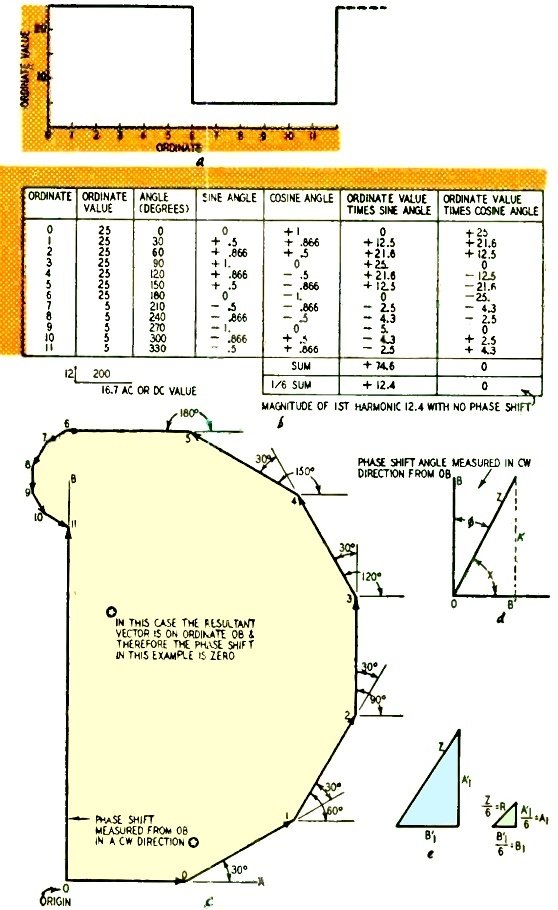
Fig. 3 - Vector diagram of a square wave and method of construction.
The first term of the equation is A0, the dc component of the wave.
Fourier analysis can of course be used to analyze a waveform with no dc component,
such as the sine wave of Fig. 2-a. In this wave, a voltage (or a current, if
you like) starts from zero and reaches a positive maximum in 90°, one-quarter of
a cycle. In the next quarter it drops to zero and in the third starts in the other
direction and reaches a maximum. In the last quarter it drops to zero and is ready
to start all over again.
To analyze the wave, we set up a number of ordinates, evenly spaced along the
cycle, to give us its value at the instants the ordinates represent. (We say "value"
because the curves may represent voltage or current.) In our examples ordinates
are placed every 30°, giving 12 ordinates a cycle. For greater accuracy more ordinates
- say one every 10° - could be set up, but every 30° is enough for most wave-shapes.
We number our ordinates from 0 to 11 (ordinate 12 is ordinate 0 since it starts
the cycle again). The table, Fig. 2-c, is then made. To find the average ordinate,
representing the dc value of the wave, we add all the values and divide by the number
of ordinates. In this case, the average value is zero, as is the case with all symmetrical
ac sine waves. Fig. 2-d shows a wave of exactly the same shape as 2-a or
-b, but with a different zero axis. Most of this wave is negative. Fig. 2-e
shows that the dc component of the wave is -14.8. This is the value a dc meter would
indicate. The next step is to determine the magnitude of the first harmonic. Mathematically
this is represented by A1, Sin x ÷ B, Cos x where
Graphically this means, to find A1, take the sum of the ordinates
each multiplied by the sine of the angle at which it occurs, and divide by half
the number of ordinates used. To find B, take the sum of each ordinate multiplied
by the cosine of the angle at which it occurs, and divide by half the number of
ordinates used.
Let us work with the square wave of Fig. 3-a. The 360° are divided into
12 intervals and the ordinate length determined. The table (Fig. 3-b) is then
made. Next the respective ordinate values are placed end to end in a vector polygon
(see Fig. 3-c) with each ordinate placed at the angle it appears in the cycle.
This takes care of the multiplication by the sines and cosines of the respective
angles at which the ordinates occur.
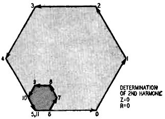
Fig. 4 - Vector diagram of a square wave's second harmonic.
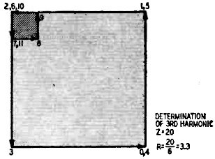
Fig 5 - Vector diagram of a square wave's third harmonic.
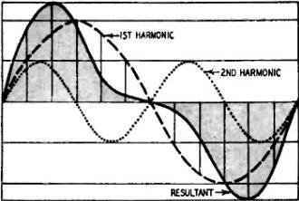
Fig. 6 - Fundamental, second harmonic and resultant frequencies.
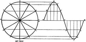
Fig. 7 - A unit circle used to construct a sine-wave drawing.
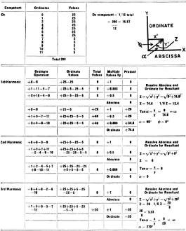
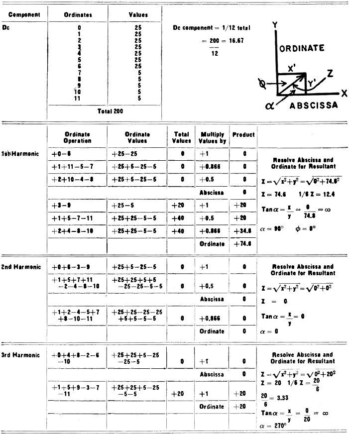
Table I - Determining Components of Waveforms (values taken from
Figs. 3, 4, and 5)
Computing Resultant Vectors
The resultant vector Z, drawn from the point of origin to the end of the last
of the ordinates, gives the total value of all the vectors and can be analyzed in
terms of its component vectors. The sum of the ordinate (vertical) values of these
is equal to the vertical value of the resultant. The sum of the abscissa (horizontal)
values of the vectors is equal to the horizontal value of the resultant. Each vector
value in the table (Fig. 3-b) times the sine of its respective angle gives
the ordinate value (A1) and each of them multiplied by the cosines of
their respective values gives the abscissa value (B1).
If the vectors do not terminate at a point on the line OB of Fig. 3-c, this
displacement is found by drawing a line from the origin (0) to the terminating point
and measuring the angle between the two lines clockwise from OB. This angle is the
phase displacement in degrees from the origin (Fig. 3-d) .
The second and third harmonics are found by drawing graphs similar to those of
Figs. 3-b and 3-c. Since the second harmonic is twice the frequency of the first,
it will go through 60° while the first harmonic goes through 30°. Thus the ordinates
are drawn at a 60° angle to each other, as in Fig. 4. The third harmonic is
three times the frequency and the quantities are 90° apart, as in Fig. 5. Measuring
our resultants, we find that the first harmonic vector is 74.6 units long, making
its value 12.4 (1/6 of 74.6). The second harmonic is zero, and the third harmonic
is 1/6 of 20, or about 3.3, in phase with the first harmonic.
So far we have dealt with positive quantities only - all our ordinates have been
measured up from the base line. In actual work true ac forms appear on both sides
of the zero axis. The same method will work, only the vector additions are more
difficult. For example take a combination of fundamental and second harmonics. To
be sure we get the right wave, we can draw a sine wave (first harmonic) (dashed
lines of Fig. 6) and another of twice the frequency (second harmonic) (dotted
lines). Then we add the two together at a large number of points, and draw the resultant
(solid line).
Now as seen from Table I, a number of our quantities are negative - measured
downward from the axis. Note that when a negative quantity is added, the angle and
distance are the same as for a positive quantity, but the line is drawn backward.
Thus a 210° quantity, instead of being drawn down and to the left at an angle of
30° from the horizontal, is drawn up and to the right.
Drawing the vector polygon for the first and second harmonics of the wave, we
find that the amplitude (peak) of the first harmonic is 10 and the second 5. Had
we started out with a single complex wave like the solid line of Fig. 6, we
would now be able to draw the two waves of which it is composed.
In drawing sine waves like the first and second harmonics in Fig. 6 - or
any combination of harmonics in any wave the reader may analyze - the unit circles
of Fig. 7 are useful. The first circle is drawn with a radius of 10, that of
the first-harmonic peak value. The second has a radius of 5, the second-harmonic
peak. The circles are divided into 30° segments, and the base of the sine wave is
laid out at the same level as the center of the circle. The circle is divided into
12 sections, one for each ordinate, 30° apart. Then a horizontal projection from
the 30° point on the circle to the 30° ordinate will give the correct amplitude
(height) for that point. The other ordinates are similarly handled and the points
connected for a sine wave.
Computing Components Arithmetically
Table I shows how the components of a wave may be determined arithmetically,
without drawing any figures. It is derived from Figs. 3, 4, and 5. First the do
component is found by adding the ordinates and dividing by 12. In the case of our
square wave, it comes to 16.7. This is the value a dc meter would read. To find
the alternating component, each value is multiplied by the sine and cosine of its
angle to find a resultant value and the phase shift. The resultant is divided by
half the number of ordinates used to find the amplitude of the component. This is
actually what we have been doing in the diagrams. For example, a line 10 units long
at an angle of 30° to the horizontal will be found to have risen 5 units.
The end of the line will be 5 units above a point 8.66 units from its origin,
the 8.66 being measured along the abscissa. The sine of the 30° angle is 0.5 and
the cosine 0.866.
It can be seen from Fig. 3 that vector 0 is entirely in the horizontal direction
and does not contribute any vertical component to the resultant vector Z. Vector
1 has a vertical component equal to the ordinate value of the wave (at 30°) times
the sine of 30°. Vector 1 has a horizontal component equal to the ordinate value
of the wave (at 30°) times cosine 30°. We can find the vertical and horizontal components
in the resultant vector by simply adding the vertical and horizontal components
of each of the respective component vectors in turn.
When adding horizontal components a vector moving toward the right on the graph
has a positive value; to the left a negative value. With vertical components a vector
moving up has a positive value; down a negative value. A chart to simplify this
procedure is shown in Table I. The values used are from Figs. 3, 4 and 5.
In our example the vertical component was 74.6 and the horizontal component was
zero. The magnitude
Z = √(x2 + y2) =
74.6. The angle that the resultant makes with the horizontal is
tan Θ = y/x, but the phase shift
is measured from the vertical (OB of Fig. 3) therefore
tan Θ = x/y. We have determined the
phase shift and what remains is to determine the amplitude of the first harmonic.
This is done by taking one-sixth the resultant
Z: 1/6Z = 74.6/6 = 12.4.
With this explanation it should be easy to follow Table I to determine the amplitude
and phase of the various harmonics, without having to draw a figure.
|