|
|||||||||||||
 |
|||||||||||||
Mathematics in Radio - Differential Calculus |
|||||||||||||
This entry level introduction of differential calculus as it applies to electronic circuit analysis appeared way back in a 1932 edition of Radio News magazine. It was written by none other than Sir Isaac Newton himself (just kidding, of course). Author J.E. Smith created an extensive series of lessons that began with simple component and voltage supply descriptions and worked up through algebraic manipulations and on finally to calculus. I remember not being the best math student in high school (OK, one of the worst), but once I got an appreciation for the power of mathematics for analyzing electronics, mechanics, physics, and even economics, my motivation level soared to where I craved more of it and ended up receiving "As" in all my college math courses. That is truly an indication that while not everyone can excel at math, the proper environment can make a world of difference. Mathematics in Radio Part Eighteen - Differential Calculus
Fig. 1 - Sinewave. Calculus and Its Application in Radio By J. E. Smith* We are learning that the study of Calculus is not as difficult as it first appeared to be and that it is essential to the understanding of advanced electrical theory and practice. The practical engineer generally asks himself to what extent the use of Calculus will enable him to advance more rapidly in his work. This is more effectively answered by the fact that a knowledge of this subject, when once appreciated, induces a confidence in one's self that is invaluable. In order to appreciate more fully the practical applications of Calculus to Radio, let us develop in more detail some of the relations in Radio theory which are already known. The study of such a subject only requires a correlation of known facts.
Fig. 2 - Slope of sinewave. We have stated previously that the differential calculus deals with the rate of change of one variable with respect to another. Let us investigate the simple sine wave of Fig. 1, in order to bring out a little more thoroughly the relationship involving the "rate of change." We have here a sine wave function of "e" or "i" which varies with the value of θ. But going a step further, the rate of change of the sine wave at any instant can be expressed in another way. Thus, with reference to Fig. 2 (a), a line PT has been drawn tangent to the sine wave at point A. The slope of such a line is defined as the ratio of 0 to a. This ratio is approximately equal to 1. Consider Fig. 2 (b), and at point B, it is noticed that the slope of the line is determined from the ratio of approximately 11 divisions to 37 divisions which is about 1/3. Now, if the line PT is drawn tangent to the curve where it goes through the zero axis at point a as shown in Fig. 3, it is apparent that its slope is greater than for points A and B. It is seen to be in the ratio of about 25 to 17, or approximately 1.5. The slope of the line drawn tangent to the curve at any point determines the rate of change of the wave. From the above analyses, the rate of change at 0 is greater than at A. In like manner, the rate of change at A is greater than at B, and for a point on the curve which is its maximum, such as E max in Fig. 1, the slope must be zero. Thus, the rate of change is maximum at zero (o) and minimum at the top of the wave (E max). The use of calculus will show this result immediately. Let the wave of Fig. 1 be expressed as follows: (I) e = E max sin θ
Fig. 3 - Slope of sinewave zero crossing.
Fig. 4 - Derivative of a sinewave shifted 90°
Fig. 5 - Current through an inductor.
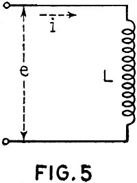
Fig. 6 - Voltage across an inductor. But it was shown in the last article that the value of the derivative at any point on the curve is equal to the slope of the line drawn tangent to the curve at that point. Let us take the derivative of (I) with respect to θ: (II) This is of the form shown to be equal to equals sin θ. Equation (II) becomes: (III) Plotting III in Fig. 4, it is noticed that calculus has determined immediately the rate of change at any instant of the sine wave. It is also in agreement with the above analyses, as it is noticed that the rate of change is maximum when the sine wave passes through zero and is at minimum when the crest of the wave has been reached. This analysis is a very important one, and further use will be made of it in later discussions. Reactive Electromotive Force Drop with Inductance Let us consider how the use of calculus shows the relation of the current with respect to the voltage in an inductive circuit. We think of the inductance of a circuit as being associated with the surrounding magnetic flux and also with the current flowing through the circuit. In considering the inductive circuit of Fig. 5, we recall that there is a magnetic flux around the coil due to the current i. The self-inductance of this circuit is simply equal to the ratio of the total magnetic flux Φ to the current i. This is expressed as: (I) L = (II) Therefore, Φ = L i If the current in Fig. 5 is changing at every instant as would be the case with an alternating current, the magnitude of the magnetic flux around the coil would likewise change. This changing magnetic flux induces an e.m.f. in the coil, and the magnitude of this induced e.m.f, "e" at any instant is equal to the rate of change of the magnetic flux with respect to time (t). This is expressed as: (III) e = The above relation can be used to advantage in connection with equation (II) in order to show the relation of the current in an inductive circuit with respect to the impressed voltage. Equation (III) tells us that we can take the derivative of equation (II) with respect to (t). Thus: (IV) Here, L is a constant, and (IV) is of the form Then (III) becomes: (V) e = L = The instantaneous value of the current is expressed by the following equation: (VI) i = Imax sin θ = Imax sin ωt Now, equation (V) tells us that we can take the derivative of equation (VI) with respect to "t". Thus: (VII) Here, I max is a constant, and (VII) is of the form
The solution of (V) thus becomes: (VIII) e = ω L Imax cos ωt This last formula, which has been easily obtained by the use of differential calculus gives us all the information that is necessary in order to show the relation of the current in the circuit of Fig. 5, with respect to the impressed voltage. From equation VIII, we recognize the reactance formula for inductance, that is, xL = 2 π f L = ω L. Plotting the instantaneous value of the current and the value of the voltage e, as obtained in equation VIII, the graph, Fig. 6, immediately informs us that the current in an inductive circuit lags behind the impressed voltage by 90°. * President, National Radio Institute.
Posted April 28, 2022 |
|||||||||||||
 |
|||||||||||||
|
|||||||||||||




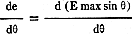
 (cv), the solution of
which has been
(cv), the solution of
which has been  . Here, E max equals C
and v
. Here, E max equals C
and v  = E max cos θ


 , the solution of which
is c
, the solution of which
is c  .
. 

|
||||||||||||||||||||||||||||||||||||