|
|||||||||||||
 |
|||||||||||||
How to Build a Crossover Network
|
|||||||||||||
Did I ever bore you with my experience building a crossover network for a set of medium power speakers (about 100 watts each) when in the USAF? Too bad I didn't have this "How to Build a Crossover Network" article from a 1968 issue of Radio-Electronics magazine handy. I'll spare you the details, but the era was 1979, and I was in tech school at Keesler AFB studying to be an Air Traffic Control Radar Repairman. Being amped up (pun intended) with electronics theory with both semiconductor and vacuum tube circuits, I was looking to cobble together a nice amplifier and a set of speakers. Back in the day, it was possible to buy the components and build your own devices for often less than buying a commercial equivalent. There was an electronics parts store right outside the base gates in Keesler, Mississippi, so I found a schematic and building article in an electronics magazine (Popular Electronics, I think) and set about procuring components. I did not know enough about impedance matching and frequency crossover networks then to design anything respectable for the woofer, midrange, and tweeters I bought at Radio Shack, in the Gulfport mall. I built the speaker enclosures in the base woodshop, using pine boards and speaker cloth for the front also bought from Radio Shack. How to Build a Crossover Network - Use a nomograph and skip the math
Crossover Network Nomograph By Max H. Applebaum An old adage states: "A chain is only as strong as its weakest link." Similarly, the frequency bandpass of an audio system is only as wide as its narrowest component. Your amplifier and speakers may separately have flat responses beyond 20 kHz, but if the wrong frequencies, in the wrong proportions, are fed to either woofer or tweeter, decreased bandwidth and or distortion may be the result. If the speakers are driven to full power ratings at frequencies outside their normal range, their voice coils may overheat. If too much low-frequency energy is fed to the high-frequency speaker, and some high-frequency energy fed to the low-frequency speaker, the overall efficiency of the unit will be reduced substantially. Obviously, a properly designed and built crossover network is not only desirable, it is necessary.
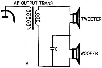
Fig. 1 - Simple crossover circuit uses a single capacitor to keep the highs out of the woofer; Slope is approximately 6 dB/octave ... just a bit too gentle for best high-fidelity work.
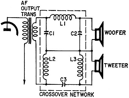
Fig. 2 - Double-pi network usually has a cutoff rate of about 18 dB/octave. This may be too steep for some applications because of excessive phase shift above and below the crossover frequency.
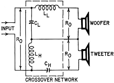
Fig. 3 - The 12 dB/octave crossover network shown here is a happy medium between circuits that do too little, and those that do too much, Phase shift two octaves above and below the crossover frequency is about midway between the 180° for 18 dB/octave and 90° for 6 dB/octave networks.
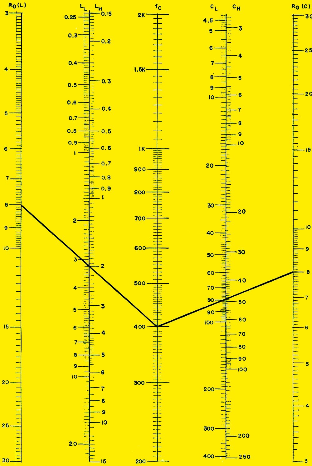
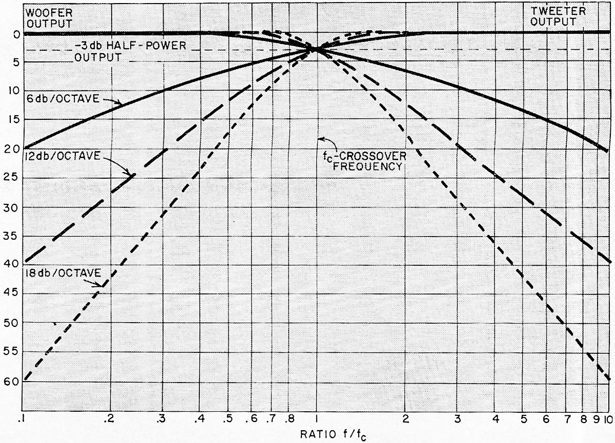
Fig. 4 - Crossover curves showing 6, 12, and 18 dB/octave rate of cutoff. The crossover frequency is the frequency of the tone both speakers reproduce equally. Circuit Function Crossover networks are built in many different configurations. The simplest type a single capacitor shunting the woofer in a series-connected woofer-and-tweeter pair (Fig. 1). A more complex type consists of two separate pi-section filters, one high-pass, the other low-pass (Fig. 2). When crossover networks are used, each speaker is supplied with a certain range of frequencies, in varying degrees of amplitude. Typical crossover plots are shown in Fig. 3; the curves represent relative attenuation versus the ratio of the actual frequency to the cutoff frequency, for various rates of attenuation. Curves are drawn for both the woofer and tweeter outputs at each rate of attenuation which results from crossover networks normally used. Crossover frequency (fc) is defined as that frequency at which the power delivered to both speakers is equal. This usually occurs with a 3-dB attenuation in power at each speaker, assuming an ideal network having no loss. The rate of attenuation is given in dB per octave, where an octave is defined as that range in which the frequency is either doubled or halved. The simple capacitor circuit of Fig, 1 provides attenuation with a gradual slope or rate of attenuation of 6 dB per octave. On the other hand, the complex network of Fig. 2 provides a sharp slope of 18 dB per octave. Each has a certain disadvantage. The single capacitor may not remove enough of the high frequencies from the woofer, while the sharp slope of the complex network may cause too much phase shift. One of the most popular networks is shown in Fig. 4-a "constant-resistance," series-connected crossover. This is a widely used arrangement, giving good fidelity and providing an attenuation of 12 dB per octave, which strikes a happy medium. While no calculations are required to use the accompanying nomograph, the following formulas are presented to give you an opportunity to double check your work. Component values are computed with the aid of equations taken from m-derived filter equations, where m = 0.6 (m-derived filter design permits either impedance or the attenuation characteristic to be predetermined ... a factor of 0.6 favors impedance match for a little more than about 80% of the audio band of frequencies, hence the reason for this particular network's "constant-resistance" characteristic) . The low-pass network (feeding the woofer) consists of series inductor LL and shunt capacitor CL. The high-pass network (feeding the tweeter) consists of series. capacitor CH and shunt inductor LH. The equations are: IMAGE HERE where fc is the crossover frequency and Ro is the nominal speaker impedance (assumed to be a pure resistance and equal for both speakers) and the output impedance of the amplifier. The solutions to these equations are rapidly found in the nomogram by merely drawing two lines. (1) From the value of fc, located on its scale, draw a straight line to the value of Ro on the outer left-hand scale. The values of LH and LL are found where the line intersects their scales. (2) CH and CL are similarly found by extending a line from the same point on the fc scale to the same value of Ro, this time on the outer right-hand scale. Note that the left-hand Ro scale is labeled R(L). This is used for the solution of the inductance values. Similarly, the right-hand Ro scale is labeled R(C). This is for the solution of capacitance values. In the example shown, Ro = 8 ohms, fc = 400 Hz, CH = 50 μF, CL = 80 μF, LL = 3.1 mH and LH = 2 mH. R-E |
|||||||||||||
 |
|||||||||||||
|
|||||||||||||

|
||||||||||||||||||||||||||||||||||||