Noise and Noise Measurements |
|
Sunshine Design Engineering Services See list of all of Joe's articles at bottom of page.
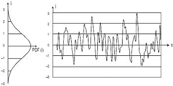
Noise and Noise Measurements By Joseph L. CahakCopyright 2013 Sunshine Design Engineering Services In today's world there is a lot of noise and interference. Noise is the cause of many communication, control and instrumentation problems and inaccuracies. This noise and interference comes from a variety of sources and has a broad spectrum of dispersion depending on the conditions of the source and the load. Einstein first brought to our attention the effect the motion of atoms or molecules have on dust particles. This was called Brownian motion. It shows the random motion of particles due to random light photons activate the electron shells of the molecular groups that then move and bump the dust particles. This random action and the loss of energy is part of the story of noise and entropy. Types of Noise There are many types of noise, Shot noise, Flicker noise, Burst noise, Transit-time noise Avalanche noise and Thermal noise to name some. See more on these at Wikipedia Electronic Noise. In addition to the thermal background noise, the environment is subjected to additional radiation noise from other sources, the sun, other cosmic objects. Solar radiation pulses impact the earth's magnetic field and influence noise into electrical systems thru magnetic interactions. Terrestrial sources such as electric devices, motors, generators, switches, surface contact, sparks or lightning can cause impulse noise. Our cars, the fire on the stove and every sources of heat or electric power also creates noise radiation in thermal losses. Our primary focus for this article will be Thermal Noise. Noise is a random distribution of energy with differing energy and time of transition components, this adds up to a broad frequency distribution of signal energy known as entropy.
Figure 1 - Random Thermal Noise Spectral Distribution - courtesy Agilent
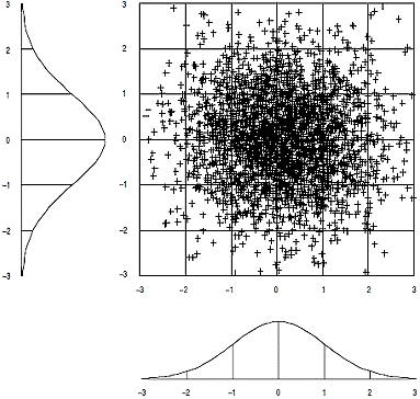
Figure 2 - Noise Spectral Distribution for Complex Modulation Signals - courtesy Agilent Spectral Noise Density Spectral Noise Density is the noise power per unit bandwidth. Expressed in Watts/Hz or dBm/Hz it represents the base noise power per unit Hz. Noise power computed for any bandwidth or temperature uses the formula
Units are typically Kelvin for temperature and dBm/Hz for logarithmic power/bandwidth or Watts/Hz for linear power/bandwidth. Power for other bandwidths can be computed from the formula
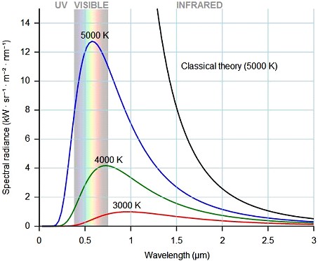
Bw1 in this case being 1 Hz and Bw2 the bandwidth the power total NpdBm covers. If we look at the black-body radiation in figure 4, it shows that the photon energy distribution as a function of wavelength, and inversely the frequency, flattens out at the lower frequencies (longer wavelengths). So while the output distribution is more Pink Noise as the level is not flat, it is close to flat in the electronic transmission frequencies. So we assume the Spectral Noise density at RF and Microwave frequencies is relatively flat at the lower thermal temperature levels. This may not always be assumed. The operator must measure the spectral signal environment to understand if any interfering signals are present for the noise figure measurement to compute properly. The shape of the spectral noise density as a function of frequency determines the color of the noise. The main colors of noise are white, pink, red (Brownian) and grey. White Noise has a flat distribution of
energy across frequency
Pink Noise, also known as flicker noise, has the mathematical representation of
Red or Brownian Noise has the mathematical
representation of
Grey Noise is random noise that has been frequency balanced to psycho-acoustically sounds flat in frequency distribution to our ears. The reader can look up Colors of Noise on Wikipedia for more information. There are a number of lesser color variants green, blue, violet, azure, black and more. Noise Power To measure noise a reference noise source is used.
There are a number of means to produce noise for reference sources. Among these are Black-body Thermal, Plasma, Electronic
and Digital. They are all , except the digital case, based on the Noise power formula Np=kTeB or
Temperature in Kelvin, Bandwidth in Hertz and Boltzmann's constant. Conversely the noise temperature can be computed
from the noise power.
These Noise power formulas are fundamental to noise sources. While the electronic noise sources may not be at a real thermal temperature in all cases, they are electrically producing noise at a higher effective noise temperature.
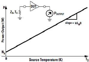
Figure 3 - Noise Power - courtesy Agilent Boltzmann's Constant The Boltzmann constant
relates how much energy something has to its temperature and is in units of Joules/K. Currently, Kelvin scale is based
off the triple point of water, which happens when water can exist as a solid, liquid, and gas at 0.01 C or 273.16 K.
The most recent value for the Boltzmann constant is
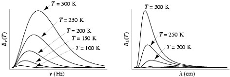
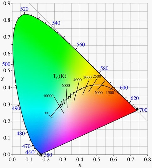
Black-Body Thermal Noise Sources Most everyone today has heard of the Big Bang. This Big Bang is the concept of the initial point our universe started from. It was an extremely high temperature and infinitely small, much, much smaller than an atomic nucleus. This expanded to the universe we see today and the Cosmic Microwave Background radiation is what we see, our rather hear today that is what is left of the energy of the Big Bang. This energy having expanded and cooled has an average temperature of just under 3.0 Kelvin. Figure 4 shows the change in radiation wavelength distribution for different temperatures and figure 5 shows the noise density at lower thermal temperatures. Figure 6 shows the spectral color change with temperature. For the 3 K CMB the spectrum will be spread to the very low microwave wavelengths and will be very flat in power vs. frequency distribution.
Figure 4 - Blackbody Radiation – courtesy Wikipedia
Figure 5 - Wein's Law at Lower Temperatures
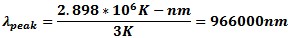
Figure 6 - Color Chart – courtesy Wikipedia Wein's Law formula can be used to calculate the wavelength peak of the black body radiation.
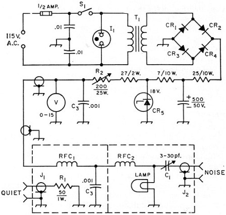
For 3 K this works out to 0.000966 M wavelength or about 30 GHz as the peak frequency of thermal radiation from cosmic background. This puts the cosmic background radiation right in the HF, VHF, UHF thru all the Microwave frequency range. The Planck Satellite has Microwave receiver bands between 80 and 1000 GHz depending on the sensors. As testament to the fact that RF and Microwave frequencies are included in this power curve of black-body radiation, in some cases a light bulb on a DC circuit with RF coupling can be used as a RF/Microwave source. See figure 7 for an example circuit. You only need to set the correct current for a certain temperature to calibrate to specific noise power outputs or ENR (Excess Noise Ratio) compared to cold noise power for the same impedance. The spectrum of the output power vs. frequency is relatively flat like white noise in the RF and Microwave region.
Figure 7 - Lamp Noise Source - see monode reference Plasma Noise Sources A plasma source is similar to the light bulb source, but uses the effective temperature of the plasma instead of the filament. These ENR's can be very high compared to other sources. An amateur plasma source would be a neon light. Just capacitively RF couple the noise off the plasma bias circuit for an easy noise source. This circuit would use a very similar circuit to figure 6, just using higher voltage to drive the plasma lamp. Electronic Noise Sources
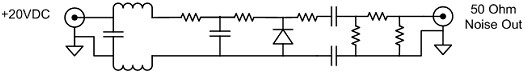
This would include Zeners, avalanche and DSP methods of generating noise output with an electrical bias input. Electronic noise sources available to amateurs include Zeners which can be used for a noise source for a antenna noise bridge, impedance bridge, noise source and more. Numerous digital signal (DAC) sources can generate pseudo-white noise that can be used for test purposes. I will go more into this later. The professional test noise sources more typically use a form of avalanche diode biased at a specific current level and temperature. Again the noise power is coupled off the bias circuit with an RF Coupling capacitor or DC coupled as in this case.
Figure 8 - Schematic of a Typical Diode Noise Source DSP or Digital Noise Sources Digitally generated noise is readily available these days from many Function Generators and can generate complex signals with added noise for C/N testing and other uses. These can greatly reduce costs for DSP SINAD and other performance test tools as we will see later. Noise Calculations
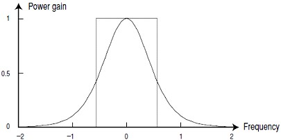
Given that any device that carries electricity generates heat, it also creates radiated noise power. In amplifiers we call this amplifier generated noise its noise figure. This gives us a measure of the signal to noise degradation of signals received and desired to be measured. ENB – Effective Noise Bandwidth ENB or Effective Noise Bandwidth is the effective power integration bandwidth or envelope of the noise power integration for total power across the spectrum. This is the ratio to correct for the effective Resolution Bandwidth of the Spectrum Analyzer or Power Measurement device with frequency selectivity to eliminate spurious signals and give an equivalent power integration bandwidth. Agilent typically uses 1.2 as the ENB integration scaling factor applied to the Resolution Bandwidth or RBW. When the Spectrum Analyzer operator selects Noise Marker the bandwidth correction is made for you.
Figure 9 - ENB Effective Noise Bandwidth - courtesy Agilent Signal to Noise Ratio The
S/N or Signal to Noise ratio is a dimensionless power ratio. It is the signal amplitude in watts compared to the Noise
power level in watts at signal off conditions. This gives some measure of signal quality or at least signal detection
capability. Every network that transports energy, in this case the RF/Microwave region has a loss or noise increase
with gain and this equates to a degradation of the S/N ratio. This measure of signal to noise degradation is called
the noise factor. This is in linear numeric scale and units relate to power ratios or signal to noise.
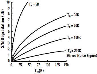
Figure 10 - Signal to Noise Degradation courtesy Agilent Technologies
Figure 11 - Signal to Noise Degradation vs. Temperature Effective in Kelvin - courtesy Agilent Minimum Detectable Signal Minimum Detectable Signal is determined by the receiver Noise Figure.
Np=kTB for T=290 K = 4*10-21 watts or -174 dBm/Hz. This is the minimum energy
in noise for a broad white spectrum distribution in the RF and Microwave region. This can also be converted from power
to noise volts in Vrms units or Arms noise current Vrms =
We now we have a basis for
Tangential Sensitivity or TSS A related signal detection parameter Tangential Sensitivity or TSS can be computed from
Noise Temperature Noise factor is related to noise temperature by
To=cold temperature and Te is effective temperature both in Kelvin.
From this we can see that to figure to a positive F, Te must exceed To. Cold Noise To depends on the desired signal to be measured. Terrestrial thermal noise limits us to greater than approximately 290K or ambient temperature of the environment. For deep space signals from gaseous clouds or other cold space targets, one would need close to 0K cooled receivers to detect the signal powers from space without being swamped by receiver noise, thus they use liquid helium coolers on these sensitive space microwave receivers. They use a 0.1K liquid He3 for the Plank satellite to measure the 3K Microwave background radiation. ENR or Excess Noise Ratio A noise source is rated by its port match and the ENR or excess noise ratio of the source and the ENR table vs. frequency calibration table. This ENR is typically expressed in dB units and is formulated from the Te and To values for the source.
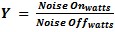
Y-Factor Y-Factor method uses the spectral analysis method to measure the spectral
density as a function of frequency and get the noise power in a specified noise bandwidth and comparing it to a cold
noise power measurement at the same bandwidth condition. This Y factor or ratio is ratio of the noise on to noise
off power ratio or
dY/dENR Another variant of the Y factor method that does not require a calibrate noise
source is the dY/dENR method. The method uses the Y and ENR measurements of 2 noise levels with and without the DUT.
The formula uses the 1st derivative of the
Note that is requires 3 or 4 measurements to get the dY and dENR and each of these measurements has error, especially if not using a good spectrum analyzer with a low noise input and level of detection. Noise Measure Noise Measure is a measure of the noise quality of the part when noise factor and gain are both considered to an infinite extension of the cascade equation, e.g. it is a measure of the system performance limit.
Receiver Noise Power Input
When making measurements or using a receiver for signal detection, the user must pay attention to the total power input to the receiver or detector/sensor to prevent overload of the receiver/sensor. Receiver gain includes antenna gain, preamp gain and total down-converted stage gain. Small signal level of broadband modulated signals can easily swamp receiver front ends. Np=kTeBG in Watts/Hz which can be converted to spectral noise density dBm/Hz. The added G factor for gain is to account for the total system noise power after receiver system gain. For wide bandwidth modulations like UWB and QAM >128 the channel power for low signal levels can be quite large and overload Spectrum Analyzer front ends. DANL or Displayed Average Noise Level This gives the relationship between the DANL of the spectrum analyzer and the analyzer noise figure of its receiver. The 1.2 is a bandwidth ENB or effective noise bandwidth factor to account for effective power integration bandwidth.
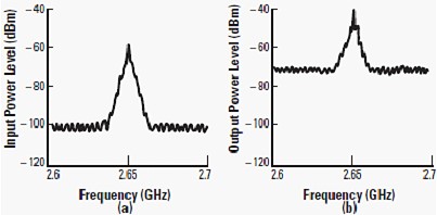
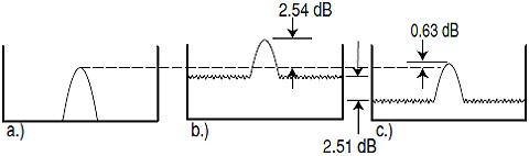
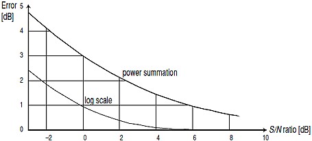
Signal to Noise Level Power Average Error When measuring CW signals close to the noise floor, as Power (mW or W) and you measure the signal and noise power and remove the signal and measure just the noise, you can figure what the actual signal power is without the added noise power. This is true even if the power is displayed as dBm.
Figure 12 - Signal to Noise Measurement Error - courtesy Agilent Signal to Noise Level Log Power Average Error When measuring CW Signals that are close to the noise floor and using log averaging the statistics are different and noise has less effect on the measurement error. The formula to figure the Signal error from the Signal and Noise total and the S/N delta in dB will give the Corrected Signal level. Agilent is using this formula and the individual noise characterization of each PSA and PXA to compute actual signal power down into the noise floor. Seemingly pulling these signals out of the Spectrum Analyzer DANL thermal noise floor is part of what Agilent is calling Noise Floor Extension.
Figure 13 - Signal to Noise Log Power Average Error - courtesy Agilent Noise Floor Extension – Agilent PSA/PXA Agilent Technologies PXA Spectrum Analyzers offer a new feature called Noise Floor Extension or NFE. This technique requires a full spectral noise density characterization of the instrument. Agilent uses the Power Average or Log Average Noise Correction techniques previous to pull the noise floor down and the signal out of the noise. Quantization Noise Error When measuring analog signals with Analog to Digital converters or generating analog signals with a DAC, there is a level of noise degradation based on the level of resolution of the ADC/DAC. The amount of the signal left after the digital “bit” voltage. The formulas for Sine or Arbitrary Wave forms are:
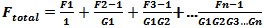
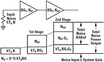
Figure 14- Quantization Noise Error Cascaded Noise Figure To compute the noise figure of cascaded network sections, the following formula is used. In noise factor and linear gain units the formula is:
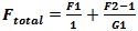
For the 2 stages case:
Use
In addition the equivalent Temperature cascade formulas are
Figure 15 - Cascade Noise Figure - courtesy Agilent Temp Corrected Noise Figure of Passive Loss
With a Loss in linear units and a Ta ambient temperature the Te effective temperature of the loss is
Use NFloss = 10log10(F) to get the loss at temperature in dB. Tl = loss temperature in Kelvin.
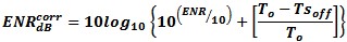
Temp Corrected ENR The temperature corrected ENR of a calibrated Noise source at a temperature other than 290 K can be computed to correct for the actual temperature offset error factor.
ENR= Noise Source ENR in dB from calibration table Ts=Noise Source actual temperature To=290 K cal temp Temp Corrected Y-Factor Noise Figure Measurement The formula for temperature corrected Y-factor noise figure measurements is
where
and
Mismatch Loss for Noise Source
Figure 16 - Noise Figure Measurement Mismatch Effects - courtesy Agilent Input Loss Correction
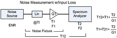
The input loss can be applied as a first order correction along with the mismatch loss for the ENR correction accounting for the input loss factor decrease in the ENR of the noise source. This is a first order correction and not as accurate s the Available Gain/Loss method described shortly. The operator must also remember to add system gain in the measurement output path into the NFM to overcome any input loss. If this is not accounted for, the noise figure meter may fail to calibrate. A first order correction can be as simple as subtracting the Effective Loss NF dB from the ENR in dB. This does not account for match or other corrections. Make sure Input Network LossdB is corrected for actual F at temperature K.
Figure 17 - Noise Measurement with Input Loss
To correct the DUT temperature for the input loss of the DUT fixture system use the equation
Output Loss Correction
The Cascaded Noise equation can be used to compute the output stage on the total system noise level into the receiver and account for this stage of loss/gain. If the device under test has a >10 of gain, then the output stage loss only impacts the gain more than the noise figure. This changes if the device under test has low gain or is lossy.
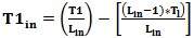
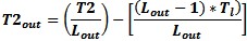
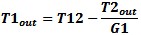
Figure 18 - Noise Measurement with Output Loss To correct the DUT temperature for the output loss of the DUT fixture system use the formulas:
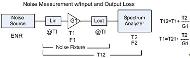
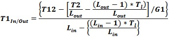
Combined Input and Output Loss Correction Combining the previous equations for input and output loss to be applied to noise figure measurements on a Noise Figure Meter when applying the input and output losses (or matching losses) to the corrected noise path measurement. The NFM would be calibrated without these losses and these input and output losses added to the DUT would be applied to the measured results to correct for the losses. This de-embeds the DUT NF from the test fixture which comprises the input loss, DUT and output loss being measured by the calibrated NFM.
Figure 19 - Noise Measurement with Input and Output Loss
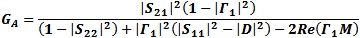
T1In/Out is the corrected DUT temperature for the input and output loss of the DUT fixture system. Input Network Available Gain/Loss The user can use a first order correction of the loss in dB and the mismatch loss of the input network. A more accurate method would be to calculate the available gain/loss from the input network s-parameters. Available gain/loss is the ratio of the power available from the 2-port network to the power available from the source. This gain is useful to calculate the network gain (or loss) of an input network to a device being tested for noise figure. This loss is the noise figure in dBF of the input network for the cascaded gain equation when making a device noise figure measurement.
with D = S11S22-S21S12 M = S11-DS'22
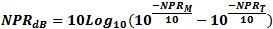
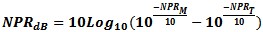
N = S22-DS'11 Noise Power Ratio Noise Power ratio gives a measure of the Infinite Intermodulation Performance of networks to digital wideband signals. It is a measure of the degradation of the measured vs. the reference test signal.
Noise Measurements Noise Measurements of Linear Devices or Non-Frequency translating To measure a typical electronic sub-assembly as an amplifier, a passive network or any other active device assemblies that are not frequency translating, the operator has several methods available to make a noise measurement. They can either use a Noise Figure Meter or a Spectrum Analyzer or a power meter with some form of filtering and amplification for the intended measurement frequency and power bandwidth and low power signal levels of noise. Noise Figure Meters Noise Figure Analyzers are basically high quality power meters with front end frequency filtering. The older Agilent 8970 series noise figure meters had a fixed 4 MHz bandwidth that it measured noise power over. If there were any interfering signals, noise figure accuracy could be greatly impacted. Noise Figure could also be impacted by narrow frequency response of the DUT affecting the power integration bandwidth. The newer Noise Figure Analyzers from Agilent have a 100 kHz to 4 MHz selectable measurement bandwidth. This does help some, but not completely eliminate issues with noise figure measurements with interfering signals and narrow bandwidth. The Noise Figure meter works best with the noise signal bandwidth being flat through the NFA bandwidth range. If sub-assembly filters or other bandwidth restricting components are within the DUT it will compromise the Noise Figure Measurement. In this case the noise figure power integration bandwidth should be less than or equal to the minimum device under test bandwidth. This will eliminate the unequal noise integration bandwidth issues of cascaded sections. The drawback is the need for amplification to overcome lower power readings with narrower bandwidth, which will add more uncertainty to the measurement.
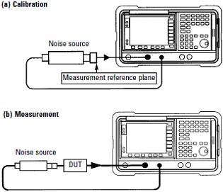
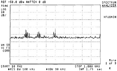
Figure 20 - Typical Noise Measurement System - courtesy Agilent An issue for noise figure meters is they do not work well with much loss between the noise source and the device under test. In practice I found about 1-2 dB loss was enough to give the 8970B NFM difficulty calibrating. One method to overcome this is to put a preamp in front of the noise figure meter to boost the noise power level to compensate for the input loss. This will result in loss of test system dynamic measurement range and possible input power saturation or overload. One needs to either measure (best) or compute the noise power into the receiver before connecting. We do not want to destroy sensitive power measurement equipment or overload it and get bad measurements. The noise measurement could be performed with a filter pre-amp and a power sensor, but is limited by the filter frequency and bandwidth and the pre-amp NF and Gain and the sensitivity of the power sensor all being fixed values. This should be an RMS or True power sensor. So this test topography could be made using other instruments besides the Noise figure meter to do the same thing. I've use everything from a power meter, Spectrum Analyzer, Vector Network Analyzer to a Scalar Analyzer for various customer/clients. Noise Figure test issues are typically boiled down to dynamic range (hi or low end gain) or spurious signals. If having trouble measuring noise figure with a noise figure meter, first diagnostic I perform is a spectrum check of the device output into the NFM and look at the noise on and noise off levels to be sure they are about what I expect to see as well.
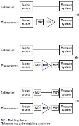
Figure 21 - Spectrum Analysis of Noise Receiver Input - courtesy Agilent If measuring devices of characteristic impedance other than 50 Ohms some means of matching the 50Ohm Noise Measurement System to the DUT under test. A Unbalanced to Unbalanced (UnUn or Coaxial) 50 ohm to 75 ohm could be used for instance, or another choice would be a 50-75 ohm minimum loss matching pad. This will add about 6 dB of loss to the path. These matching losses must be accounted for in the cascade noise math to compute the correct noise figure of the DUT, again a preamp into the receiver may be necessary to have the correct noise power levels for accurate measurements.
Figure 22 - Noise Figure with Matching to DUT - courtesy Agilent Noise Measurements by Y-Factor Spectral Analysis The issues mentioned above using a Noise Figure Meter, such as, spurious signal or detector dynamic power range are significantly overcome when using a spectrum analyzer. Where the older spectrum analyzers had slow sweep response and high input noise figures, today's analyzers are much faster, more accurate and have far better front ends and lower noise figures when Preamps are added to the front ends. Using a spectrum analyzer the test frequency can be easily moved to quieter areas to make the noise measurement. Many modern spectrum analyzers have the Y-Factor capability built in and have a drive for the noise source and the firmware to make the calculation.
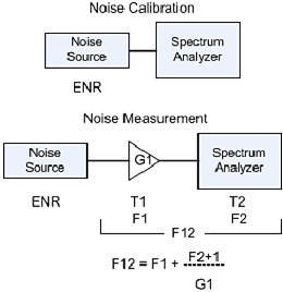
We begin the Y factor measurement by looking at the spectrum analyzer and its characteristics. First set the spectrum analyzer to sample detector at the lowest Resolution Bandwidth that gives reasonable sweep time. Place the Spectrum Analyzer in Video Averaging mode and get the noise floor average across frequency or DANL in dB. This is related to the Spectrum Analyzer's noise figure and is a measure of the sensitivity of the analyzer. Knowing the Spectrum Analyzer DANL and looking at the Noise Source with Noise ON, if we can see the jump in noise floor of the spectrum analyzer, we know we will be able to measure the Noise On and Noise Off with the DUT in the measurement system provided the DUT has a reasonable gain (>10 dB). We only need the DUT Noise On and Off measurement and the ENR of the noise source to compute the Noise Figure. We know the ENR of the source (Calibration Noise On/Noise Off), so don't need to measure it. But if the Noise On measurement of the Noise Source is more than 10 dB above the DANL of the Spectrum Analyzer, you can de-embed a reasonable accuracy on the Noise Source ENR.
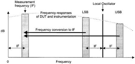
Figure 23 - Spectrum Analyzer Noise Measurement When measuring a frequency linear device such as an amp, filter, etc. the ENR used is the interpolated ENR value for the RF frequency of interest ratioed between the ENR table values above and below frequency measured. They are usually calibrated every GHz maybe 10 MHz and 100 MHz at the low frequency end. When measuring frequency translational devices such as Mixers, Receivers, Multipliers the ENR of the RF input is used and the measurement is made at the IF Freq or Vice-versa if the frequency conversion goes the other way and there may be sidebands involved or both sidebands. These need to be considered to make the measurement properly depending on the frequency conversion topology of the DUT. Noise Measurements of Frequency Translating (Mixer) Measurements The Noise Figure Analyzer also makes complex frequency translating and single sideband measurements much easier. The analyzer takes care of the ENR factors at frequency and also the LO frequency for the test. When measuring the Noise Figure of a frequency translating device such as a mixer, converter, doubler, tripler or other means of translating a signal from one frequency to another, a similar technique is used in that you know the noise power of the source hot and cold at the RF frequency being input or received. Then from the output Noise On and Noise Off measurement thru the DUT the converted signal noise degradation can be measured. Even though the measurement is made at a different frequency the power rations are the same and the ENR used is at the frequency of input to the device under test. Noise Figure Meters can be used to semi-automate these measurements by programming in the type of conversion Up-conversion or down-conversion. If the LO being used is above or below the RF frequencies or the IF being used as the input RF signal. This will determine if the RF, IF or LO are CW or swept and it the signal being converted to will sweep up or down in frequency. This is all important information for the proper path loss corrections for the signals input and output for the corrected Noise Figure of the measurement. In addition, one must know if you are measuring a single or double sideband device. If you are measuring an SSB device the actual noise figure will be 3dB higher, as you are only measuring half the input signal power.
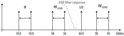
Figure 24 - Mixer Frequency Plan - Fixed LO - courtesy Agilent
Figure 25 – Mixer Noise DSB/SSB Measurements - courtesy Agilent When using the NFM, filters may be necessary to eliminate spurious signals. Spectrum Analysis Y-factor is ideally suited for noise figure measurement on frequency translating devices as spurious signal avoidance is much easier. We re-iterate that when measuring frequency translational devices such as Mixers, Receivers, Multipliers the ENR of the RF input is used and the measurement is made at the IF Freq or Vice-versa if the frequency conversion goes the other way and there may be sidebands involved or both sidebands. These need to be considered to make the measurement properly depending on the frequency conversion topology of the DUT.
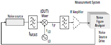
Figure 26 - Mixer Noise Figure Test - courtesy Agilent Cold Power Noise Measurement
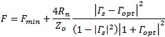
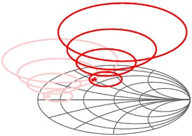
This method uses the basic cascaded noise formula to derive the noise power from an input termination thru the DUT and into the noise measurement device. By measuring this output power and knowing the input thermal power by the kTeBw formula for the watts of the defined bandwidth, we can then derive the F for the DUT under test. The high speed RFIC testers like this method, as it takes a lot less time; even if has bandwidth, match, gain/loss accuracy of switched paths and contacts repeatability and match etc. It is still very fast. You only measure one cold power sweep, not one hot and one cold as with the Y-Factor or NFM methods although the accuracy is much worse. Active Device Noise Characterization for Design Part of designing active device gain blocks for low noise front end amplifiers is to understand the noise and gain characteristics over a range of input matches. By having a test setup with integrated Vector Network Analyzer for S-Parameters and a Noise Source with input tuning stubs to match the input of hthe device the Fmin and Rs and constant noise circles and gain circles and center can be determined to aid designs using the device for better performance. By varying the match and measuring the DUT under the input match conditions and de-embedding the pre-calibrated tuner network response to get the raw device performance parameters which can be modeled by the formula. In figure 27 the pink circles of the paraboloid show a different frequency than the red circles.
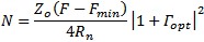
Figure 27 - Noise Match Performance Paraboloid – courtesy BSW Inc. The center of the paraboloid of noise performance on the smith chart load display is calculated with the formula:
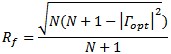
The circles of constant noise performance are calculated with the formulas:
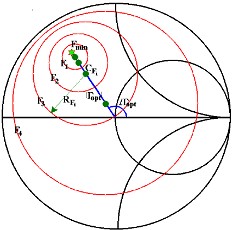
The Noise Factor at each of the circle boundaries:
Figure 28 - Noise Circles on the Smith Chart – courtesy BSW Inc. Other Noise Test Methods Noise Source as Infinite Bandwidth Signal Source
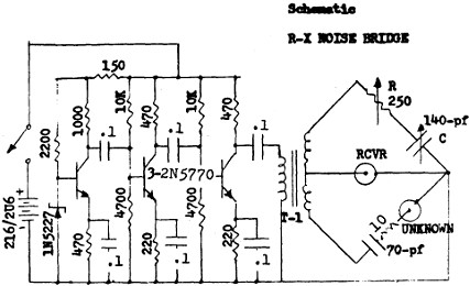
A noise source with an amplifier to increase the noise level can be used as effectively a wideband signal source. Take the wideband noise power from a noise source and pass it thru a filter, I can integrate the spectral response by averaging the output on a Spectrum Analyzer and get the filter response envelope within a short time with increasing accuracy as the averages build in count. Noise Bridge The noise bridge is a measurement instrument using a broadband RF noise source such as Zeners, or resisters, neon lamps or other broadband noise sources. Then boost the power level with an amplifier and inject into a balanced bridge. The bridge resistance and reactance tuning for nulling allows the operator to figure a system or antenna characteristic impedance so the antenna can be balanced for best power transfer. The bridge resistor of 0-250 Ohms and 0-140 pF is balanced against a 70 pF capacitor and 10 Ohm resistor and the unknown load of the antenna or other network. The 250 Ohms is to balance against network impedance of typically 20-200 Ohms range and the 140 pF variable tuning capacitor balances against 70pF in the other arm to give a +/-70 pF reactance tuning range. This gives most communication folks a good practical and cheap tool to get matching information on networks and their antennas.
Figure 29 – Palomar Noise Bridge Schematic – courtesy Palomar Technologies Noise and Antenna Gain
While researching noise measurements I found this info on antenna measurements of interest. The noise spectral density measured at the antenna output compared to the ambient thermal noise level (kTB) gives a measure antenna gain factor. Noise being infinite bandwidth this gain factor covers a broad frequency range, so it gives an easy and simple means to measure the wideband antenna gain performance. Noise for C/N or Eb/No Transceiver Performance Measurements Using an RF Noise source and providing power amplification to produce known level of
noise to couple with signal sources of known level gives the capability to test Transceivers for the Carrier to Noise
level performance testing. There are variants of this that can test the Eb/No (Energy per Bit to Noise Level) when
the data bit rate information is added to the calculation. Eb/No is related to C/N by the equation
Figure 30 - Carrier to Noise to BER Curves - courtesy Agilent Noise for Jamming The Noise source taken to an extreme with huge power amplifiers can be used to flood an area with high level of false ambient RF noise and jam all signals in that area with such high Noise levels that most all receiver systems will fail to operate properly. It is my understanding the services use 750 kW TWT's to flood the engagement areas with noise to jam. This power of 88 dBF of Noise power is equal to ~1.83*1011 K, so this is a very hot source indeed. Signal to Noise (S/N) Measurement This is a measure of the signal level over the base average noise floor of the receiver system. The average peak of the signal is compared to the average noise floor level and the difference is expressed in dB relative difference. Noise for in-circuit testing and calibration Noise can be used as in an in-circuit Built In Self Test or BIT or BIST. This can give several performance parameters such as S/N, gain an sometimes more for the device the noise injector is built into for this purpose. SINAD SINAD is a means to measure signal to noise and Distortion
quality with a simple instrument. The power of the noise and distortion with the Signal and without to determine the
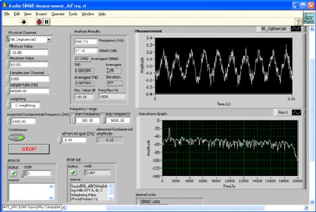
Figure 31 - 20 kHz Audio Noise SINAD
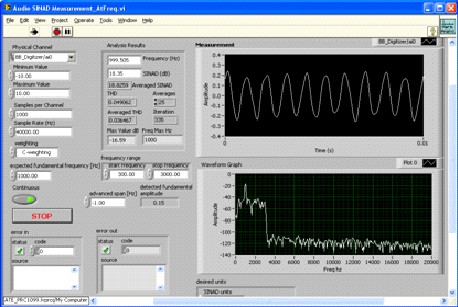
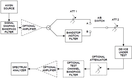
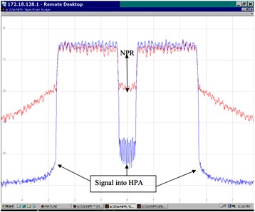
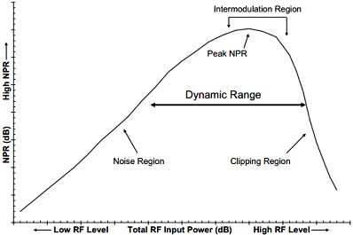
Figure 32 - 3 kHz Audio Noise SINAD Noise Power Ratio This measurement can be useful in specialized cases for measuring and determining spectral regrowth of broadband digital systems (amps, receiver, transmitters, etc.). The spectral emissions masks of most communication standards have spectral masks that must be met to be approved for use. To do this, amplifiers and other devices have to control spectral regrowth from intermodulation products. A Noise Power Ratio Analyzer creates a noise source, with a deep notch band reject filter to cut a gap of some bandwidth in the broadband noise sources. When this reference test signal is sent thru the device under test, the intermodulation products from this infinite source created Infinite Intermodulation Products IIP's that fill the noise gap. The new level with the DUT performance is compared to the old notch level gives a measure of the IIP performance and an indication of the devices contribution to spectral regrowth.
Figure 33 - Noise Power Ration Test System
Figure 34 - Noise Power Ratio Signals
Figure 35 - Noise Power Ratio Performance Curve of Amp - courtesy Agilent Conclusion
We have reviewed Noise and Noise Measurements and its many uses. We showed many of the Noise formulas and uses for Noise as well as important uses for noise. We will see new receiver technology to glean weak signals even further out of the noise background to extend our communication reach even further than is now possible. Voyager1 has now passed the boundary of the Heliosphere. Our technology to receive these faint signals improves year after year. We are still digging Voyager's signal out of the noise with Silicon on Sapphire semiconductors and Parametric Amplifiers that work on near magic to get these infinitesimal signals out of the ether. The technology to detect these signals did not exist when these spacecraft were first sent up to space. The measurement of the Cosmic Microwave Background or CMB may open new knowledge about our universe on the largest scale. Who could have known the reach of noise on our knowledge? What we started out studying to understand may end up telling us something about our place in the universe, the fate of that universe. The patterns of noise show us the acoustic signature at the point of rapid inflation at the birth of the big bang, which created the imprint for future matter (galaxy) distribution of the universe. Scientists have refined the age of the universe, how fast it is expanding and cosmic constants. The analysis of the size scale of the noise temperature fluctuations in the CMB tells us about the makeup of the universe and the ratio of Dark energy, dark matter and ordinary matter. The signatures on noise temperature of the universe are also being looked at for patterns representing the possibility of multiple universes and partners to ours bumping into our universe.
Clearly noise has much to teach us about many things and is of great use, in addition to being the bane of communications.
Sunshine Design Engineering Services 23517 Carmena Rd Ramona, CA 92065 760-685-1126 Featuring: Test Automation Services, RF Calculator and RF Math/Noise and S-Parameter Library (DLL & LLB)
References
Sunshine Design Engineering Services is located in the sunny San Vicente Valley near San Diego, CA, gateway to the mountains and skies. Are you looking for new things to design, program or create and need assistance? I offer design services with specialties in electronic hardware, CAD and software engineering, and 25 years of experience with Test Engineering services in RF/microwave, transceiver and semiconductor parametric test, test application program development, automation programs, database programming, graphics and analysis, and mathematical algorithms. See also: - Noise and Noise Measurements - Measuring Semiconductor Device Input Parameters with Vector Analysis - Computing with Scattering Parameters - Measurements with Scattering Parameters - Ponderings on Power Measurements - Scattered Thoughts on Scattering Parameters Sunshine Design Engineering Services 23517 Carmena Rd Ramona, CA 92065 760-685-1126 Featuring: Test Automation Services, RF Calculator and S-Parameter Library (DLL & LLB)
Posted December 15, 2013 |
 to convert between Noise Power and Temperature. See figure3 for Te/Np curve.
 .
.
 .
.
 .
It has a decreasing energy per Hz as frequency increases.
.
It has a decreasing energy per Hz as frequency increases.  .
It has faster decreasing energy per Hz as frequency increases as pink noise. These first three noise colors are considered
power-law noise as they follow a power law noise energy/frequency distribution White having a 0 exponent, pink a 1
and Brown an exponent of 2.
.
It has faster decreasing energy per Hz as frequency increases as pink noise. These first three noise colors are considered
power-law noise as they follow a power law noise energy/frequency distribution White having a 0 exponent, pink a 1
and Brown an exponent of 2.
 =
=
 in SI base units with an uncertainty of Ur=0.71ppm about half of the last best measurement. See
 .
The
.
The
 is the signal to noise ratio of the system calibration. The
 is
the signal to noise ratio of the system and DUT total response. This is more typically used in the Log format Noise
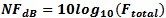
Figure in NFdB which can be computed from the formula
is
the signal to noise ratio of the system and DUT total response. This is more typically used in the Log format Noise
Figure in NFdB which can be computed from the formula
 .
The inverse of this can be computed from
.
The inverse of this can be computed from
 or Irms =

 or
or  when
the temperature of the system under test is not at Te=290K.For a receiver with a S/N performance level the MDS formula
adds the S/N factor
when
the temperature of the system under test is not at Te=290K.For a receiver with a S/N performance level the MDS formula
adds the S/N factor

 or
or
 or Te = To(F-1).
 for when user is using noise figure in log units.
 or
or 
 or
or  with
To=290K
with
To=290K off with Np on must be greater than Np off to compute a noise figure. Then the Y ratio can be used to compute the
Noise Figure in dB. Be sure to use sample detector mode when making these measurements. Video Averaging will reduce
the specular noise by averaging across frequency to smooth to the video average.
off with Np on must be greater than Np off to compute a noise figure. Then the Y ratio can be used to compute the
Noise Figure in dB. Be sure to use sample detector mode when making these measurements. Video Averaging will reduce
the specular noise by averaging across frequency to smooth to the video average. or
or 
 from
which we derive
from
which we derive 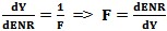 .
.
 in
linear units of F=Noise Factor and G=Gain in linear units.
in
linear units of F=Noise Factor and G=Gain in linear units.


 for
Arbitrary Waveforms
for
Arbitrary Waveforms for
Sine Waveforms
for
Sine Waveforms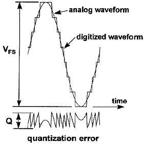
 or
or  or
or 
 to convert to dBF. This can be used to compute the noise figure of a DUT embedded inside a test fixture. Keep in mind
T can be substituted in for F using Te=To(F-1) in the equation for cascaded noise calculations. We will see these
formulas again with input and output loss correction of DUT measurements. We will also see this in the cold power
noise measurement technique.
to convert to dBF. This can be used to compute the noise figure of a DUT embedded inside a test fixture. Keep in mind
T can be substituted in for F using Te=To(F-1) in the equation for cascaded noise calculations. We will see these
formulas again with input and output loss correction of DUT measurements. We will also see this in the cold power
noise measurement technique.
 from
which we compute the noise factor
from
which we compute the noise factor  .
.


 . The + and – represent the max and minimum mismatch for the measurement mismatch loss of power measured. ρg and
ρl are the generator and load reflection coefficient. This would be an input loss direct error factor
on the measurement that is F1 in the cascade noise equation along with the input network loss added for the total
loss.
. The + and – represent the max and minimum mismatch for the measurement mismatch loss of power measured. ρg and
ρl are the generator and load reflection coefficient. This would be an input loss direct error factor
on the measurement that is F1 in the cascade noise equation along with the input network loss added for the total
loss.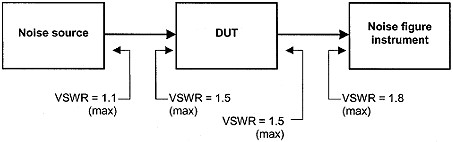

 T1=DUT, Lin = Loss, Tl = Loss effective temperature in K.
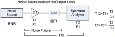
 n
n

 with
ENB=Rcvr Noise BW, fb=bit rate
with
ENB=Rcvr Noise BW, fb=bit rate 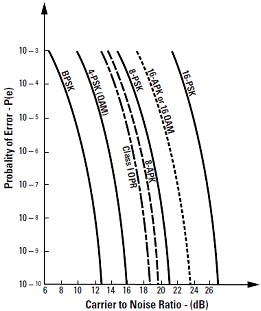
 .
In practice the power is detected for the input signal for the S+N+D. For the N+D the signal is filtered with a tight
signal frequency filter and the Noise and Distortion components are left to use to divide the total power by for the
resulting SINAD. When measuring a receiver audio output the bandwidth of the SINAD measuring instrument can give varying
results depending on how wide the noise floor extends in frequency. If the audio output is integrated for SINAD over
a 3 kHz bandwidth vs. over a say 20 kHz bandwidth the SINAD will be much lower for the wideband noise case
verse the narrow band audio noise case. Most receiver audio channels are not very wide in bandwidth for signal
transmission efficiency. So, if having trouble with a receiver, measuring SINAD, check the measurement bandwidth.
In the case shown in figure 31 and 32, the impact of the wideband audio noise on a SINAD measurement is demonstrated.
In this case SINAD went from 16.4 dB in the 20 kHz noise case to 18.4 dB in the 3 kHz noise bandwidth
case. In both cases the S/N ratio was approximately equal. So the difference was just from the added noise bandwidth.
.
In practice the power is detected for the input signal for the S+N+D. For the N+D the signal is filtered with a tight
signal frequency filter and the Noise and Distortion components are left to use to divide the total power by for the
resulting SINAD. When measuring a receiver audio output the bandwidth of the SINAD measuring instrument can give varying
results depending on how wide the noise floor extends in frequency. If the audio output is integrated for SINAD over
a 3 kHz bandwidth vs. over a say 20 kHz bandwidth the SINAD will be much lower for the wideband noise case
verse the narrow band audio noise case. Most receiver audio channels are not very wide in bandwidth for signal
transmission efficiency. So, if having trouble with a receiver, measuring SINAD, check the measurement bandwidth.
In the case shown in figure 31 and 32, the impact of the wideband audio noise on a SINAD measurement is demonstrated.
In this case SINAD went from 16.4 dB in the 20 kHz noise case to 18.4 dB in the 3 kHz noise bandwidth
case. In both cases the S/N ratio was approximately equal. So the difference was just from the added noise bandwidth.