Module 12 - Modulation Principles
Pages i,
1-1,
1-11,
1-21,
1-31,
1-41,
1-51,
1-61,
1-71,
2-1,
2-11,
2-21,
2-31,
2-41,
2-51,
2-61,
3-1,
3-11,
3-21,
3-31, AI-1, Index, Assignment 1, 2
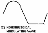
Figure 2-27C. - Overmodulation of a carrier. NONSINUSOIDAL MODULATING WAVE. Observe the modulating square wave in figure 2-28. Remember that it contains an infinite number of odd
harmonics in addition to its fundamental frequency. Assume that a carrier has a frequency of 1 megahertz. The
fundamental frequency of the modulating square wave is 1 kilohertz. When these signals heterodyne, two new
frequencies will be produced: a sum frequency of 1.001 megahertz and a difference frequency of 0.999 megahertz.
The fundamental frequency heterodynes with the carrier. This is also true of all harmonics contained in the square
wave. Side frequencies associated with those harmonics will be produced as a result of this process. For example,
the third harmonic of the square wave heterodynes with the carrier and produces sideband frequencies at 1.003 and
0.997 megahertz. Another set will be produced by the fifth, seventh, ninth, eleventh, thirteenth, fifteenth,
seventeenth, and nineteenth harmonics of the square wave, and so on to infinity.
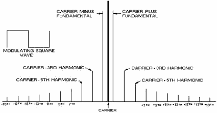
Figure 2-28. - Spectrum distribution when modulating with a square wave.
Look at figure 2-28 and observe the relative amplitudes of the sidebands as they relate to the amplitudes of
the harmonics contained in the square wave. Note that the first set of sidebands is directly related to the
amplitude of the square wave. The second set of sidebands is related to the third harmonic content of the square
wave and is 1/3 the amplitude of the first set. The third set is related to the amplitude of the first set of
sidebands and is 115 the amplitude of the first set. This relationship will apply to each additional set of
sidebands. 2-31
View (A) of figure 2-29 shows the carrier modulated with a square wave. In view (B) the modulating
square wave is increased in amplitude; note that the RF peaks increase in amplitude during the positive
alternation of the square wave and decrease during the negative half of the square wave. In view (C) the amplitude
of the square wave is further increased and the amplitude of the RF wave is almost 0 during the negative
alternation of the square wave.
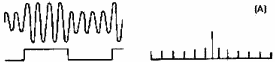
Figure 2-29A. - Various square-wave modulation levels with frequency-spectrum carrier and
sidebands.
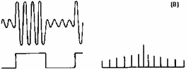
Figure 2-29B. - Various square-wave modulation levels with frequency-spectrum carrier and
sidebands.
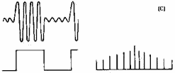
Figure 2-29C. - Various square-wave modulation levels with frequency-spectrum carrier and
sidebands.
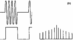
Figure 2-29D. - Various square-wave modulation levels with frequency-spectrum carrier and
sidebands.
2-32
Note the frequency spectrum associated with each of these conditions. The carrier amplitude remains
constant, but the sidebands increase in amplitude in accordance with the amplitude of the modulating square wave. So far in pulse modulation, the same general rules apply as in AM. In view (C) the amplitude of the square wave of
voltage is equal to the peak voltage of the unmodulated carrier wave. This is 100-percent modulation, just as in
conventional AM. Note in the frequency spectrum that the sideband distribution is also the same as in AM. Keep in
mind that the total sideband power is 1/2 of the total power when the modulator signal is a square wave. This is
in contrast to 1/3 the total power with sine-wave modulation. Now refer to view (D). The increase of the
square-wave modulating voltage is greater in amplitude than the unmodulated carrier. Notice that the sideband
distribution does not change; but, as the sidebands take on more of the transmitted power, so will the carrier. Pulse Timing Thus far, we have established a carrier and have caused its peaks to
increase and decrease as a modulating square wave is applied. Some pulse-modulation systems modulate a carrier in
this manner. Others produce no RF until pulsed; that is, RF occurs only during the actual pulse as shown in view
(A) of figure 2-30. For example, let's start with an RF carrier frequency of 1 megahertz. Each cycle of the RF
requires a certain amount of time to complete. If we allow oscillations to occur for a given period of time only
during selected intervals, as in view (B), we are PULSING the system. Note that the pulse transmitter does not
produce an RF signal until one of the positive-going modulating pulses is applied. The transmitter then produces
the RF carrier until the positive input pulse ends and the input waveform again becomes a negative potential. 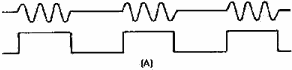
Figure 2-30A. - Pulse transmission.
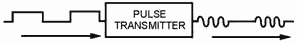
Figure 2-30B. - Pulse transmission.
Refer back to figure 1-41 and the over-modulation discussion in chapter 1. You will notice that the
overmodulation wave shape of view (D) in figure 2-29 and the pulse-modulation wave shape of figure 2-30, view
(B), are very similar to figure 1-41. Actually, both figure 1-41 and view (D) of figure 2-29 result from
overmodulation. Even though the output of the pulse transmitter in figure 2-30 looks like overmodulation, it is
not; rather, it is pulsed.
2-33
However, the frequency spectrums are similar. Sideband distributions are similar, but not identical,
since the pulse transmitter in figure 2-30 is gated on and off instead of being modulated by a square wave as was
the case in view (D) of figure 2-29. Remember, in pulse modulation the sidebands produced to accompany the
carrier during transmission are directly related to the harmonic content of the modulating wave shape. In figure
2-31, (view A, view B and view C), observe the square and rectangular wave shapes used to pulse modulate the same
carrier frequency in each of the three views.
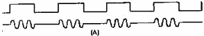
Figure 2-31A. - Varying pulse-modulating waves. 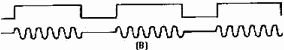
Figure 2-31B. - Varying pulse-modulating
waves. 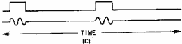
Figure 2-31C. - Varying pulse-modulating waves.
Let's take note of some timing relationships in the three modulating sequences in figure 2-31: •
the time for the RF cycle is the same in each case • the number of cycles occurring in each group is
different • the ratio between transmitting and non-transmitting time varies • the transmitter
produces an RF wave four times in view (A), three transmission groups in view (B), and only two in view
(C) • RF is generated only during the positive pulses 2-34
IIn figure 2-32, observe the relative time for individual RF cycles. The time for each cycle is the
same in views (A) and (B). Since this time is the same, we can assume that the carrier frequency is the same. But
in view (C) the time for each cycle is about half that in views (A) and (B). Therefore, the frequency of the
carrier in view (C) is nearly twice that of the other two. This illustration shows that carrier frequencies in
pulse systems can vary.
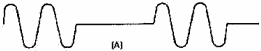
Figure 2-32A. - Carrier frequency. 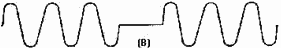
Figure 2-32B. - Carrier frequency. 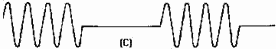
Figure 2-32C. - Carrier frequency.
The carrier frequency is not the only frequency we must concern ourselves with in pulse systems. We must also
be concerned with the frequency that is associated with the repetition rate of groups of pulses. Figure 2-33 shows
that a specific time period exists between each group of RF pulses. This time is the same for each repetition of
the pulse and is called the PULSE-REPETITION TIME (PRT). To find out how often these groups of pulses occur,
compute PULSE-REPETITION Frequency (PRF) using the formula:

2-35
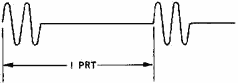

Figure 2-33. - Pulse-repetition time (PRT). Just remember that the pulse-repetition time is the time it takes for a pulse to recur, as shown in
figure 2-34. The duration of time of the pulse (a) plus the time when no pulse occurs (b) equals the total
pulse-repetition time.
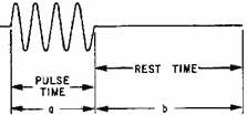

Figure 2-34. - Pulse cycles.
The time during which the pulse is occurring is called PULSE DURATION (PD) or PULSE WIDTH (PW), as shown in
figure 2-35. As you will soon see, pulse width is important in pulse modulation. 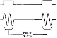
Figure 2-35. - Pulse width (PW). 2-36
The time we have been referring to as the time of no pulse, or nonpulse time, is referred to as REST
TIME (rt). The duration of this rest time will determine certain capabilities of the pulse-modulation system. The
pulse width is the time that the transmitter produces RF oscillations and is the actual pulse transmission time.
During the nonpulse time, shown in figure 2-36, the transmitter produces no oscillations and the oscillator is cut
off.
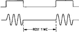
Figure 2-36. - Rest time (RT).
Some pulse transmitter-receiver systems transmit the pulse and then rest, awaiting the return of an echo. Rest
time provides the system time for the receive cycle of operation. Power in a Pulse System When discussing power in a pulse-modulation system, we have to consider PEAK Power and AVERAGE Power. Peak
power is the maximum value of the transmitted pulse; average power is the peak power value averaged over the
pulse-repetition time. Peak power is very easy to see in a pulse system. In figure 2-37, all pulsed wave shapes
have a peak power of 100 watts. Also note that in views (A), (B), and (C) the pulse width is the same, even though
the carrier frequency is different. In these three cases average power would be the same. This is because average
power is actually equal to the peak power of a pulse averaged over 1 operating cycle. However, the pulse width is
increased in view (D) and we have a greater average power with the same PRT. In view (E) the decreased pulse width
has decreased average power over the same PRT.
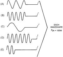
Figure 2-37. - Peak and average power. 2-37
Use these simple rules to determine power in a pulsed-wave shape: • Peak power is the maximum
power reached by the transmitter during the pulse. • Average power equals the peak power averaged over one
cycle. Duty Cycle In pulse modulation you will need to know the percentage of time
the system is actually producing rf. For example, let's say that a pulse system is transmitting 25 percent of the
time. This would mean that the pw is 1/4 the t. For every 60 minutes we operate the pulse system, we actually
transmit a total of only 15 minutes. The DUTY Cycle is the ratio of working time to total time for
intermittently operated devices. Thus, duty cycle represents a ratio of actual transmitting time to transmitting
time plus rest time. To establish the duty cycle, divide the pw by the PRT of the system. This yields the duty
cycle and is expressed as a decimal figure. With this information, we can figure percentage of transmitting time
by multiplying the duty cycle by 100. Applications of Pulse Modulation Pulse
modulation has many applications in the transmission of intelligence information. In telemetry, for example, the
width of successive pulses may tell us humidity; the changing of the rest time may tell us pressure. In other
applications, as you will see later in this text, the changing of the average power can provide us with
intelligence information. In radar a pulse is transmitted and travels some distance to a target where it
is then reflected back to the system. The amount of time it takes provides us with information that can be
converted to distance. Telemetry and radar systems use the principles of pulse modulation described in
this section. Let's quickly review what has been presented: • Pulse width (pw) - the duration of time
RF frequency is transmitted • Rest time (RT) - the time the transmitter is resting (not transmitting)
• Carrier frequency - the frequency of the RF wave generated in the oscillator of the transmitter •
Pulse-repetition time (PRT) - the total time of 1 complete pulse cycle of operation (rest time plus pulse
width) • Pulse-repetition frequency (PRT) - the rate, in pulses per second, that the pulse occurs •
Power peak - the maximum power contained in the pulse • Average power - the peak power averaged over 1
complete operating cycle • Duty cycle - a decimal number that expresses a ratio in a pulse modulation
system of transmit time to total time 2-38
Pulse modulation will play a major part in your electronics career. In one way or another, you will
encounter it in some form. The function of the particular system may involve many variations of the
characteristics presented here. We will now look at some specific applications of pulse modulation in radar and
communications systems.
Q-14. Overmodulating an RF carrier in amplitude modulation produces a waveform which is similar to what
modulated waveform? Q-15. What is PRT? Q-16. What is nonpulse time? Q-17. What is
average power in a pulsed system? Radar MODULATION Radio frequency energy in
radar is transmitted in short pulses with time durations that may vary from 1 to 50 microseconds or more. If the
transmitter is cut off before any reflected energy returns from a target, the receiver can distinguish between the
transmitted pulse and the reflected pulse. After all reflections have returned, the transmitter can again be cut
on and the process repeated. The receiver output is applied to an indicator which measures the time interval
between the transmission of energy and its return as a reflection. Since the energy travels at a constant
velocity, the time interval becomes a measure of the distance traveled (RANGE). Since this method does not depend
on the relative frequency of the returned signal, or on the motion of the target, difficulties experienced in CW
or fm methods are not encountered. The pulse modulation method is used in many military radar applications. Most radar oscillators operate at pulse voltages between 5 and 20 kilovolts. They require currents of several
amperes during the actual pulse which places severe requirements on the modulator. The function of the high-vacuum
tube modulator is to act as a switch to turn a pulse ON and ofF at the transmitter in response to a control
signal. The best device for this purpose is one which requires the least signal power for control and allows the
transfer of power from the transmitter power source to the oscillator with the least loss. The pulse modulator
circuits discussed in this section are typical pulse modulators used in radar equipment. Spark-Gap
Modulator The SPARK-GAP Modulator consists of a circuit for storing energy, a circuit for rapidly
discharging the storage circuit (spark gap), a pulse transformer, and an ac power source. The circuit for storing
energy is essentially a short section of artificial transmission line which is known as the PULSE-forMING Network
(PFN). The pulse-forming network is discharged by a spark gap. Two types of spark gaps are used: FIXED GAPS and
ROTARY GAPS. The fixed gap, discussed in this section, uses a trigger pulse to ionize the air between the contacts
of the spark gap and to initiate the discharge of the pulse-forming network. The rotary gap is similar to a
mechanically driven switch. A typical fixed, spark-gap modulator circuit is shown in figure 2-38. Between
trigger pulses the spark gap is an open circuit. Current flows through the pulse transformer (T1), the
pulse-forming network (C1, C2, C3, C4, and L2), the diode (V1), and the inductor (L1) to the plate supply voltage
(Eb). These components form the charging circuit for the pulse-forming network. 2-39
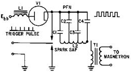
Figure 2-38. - Fixed spark-gap modulator. The spark gap is actually triggered (ionized) by the combined action of the charging voltage across the
pulse-forming network and the trigger pulse. (Ionization was discussed in NEETS, Module 6, Introduction to
Electronic Emission, Tubes and Power Supplies.) The air between the trigger pulse injection point and ground is
ionized by the trigger voltage. This, in turn, initiates the ionization of the complete gap by the charging
voltage. This ionization allows conduction from the charged pulse-forming network through pulse transformer T1.
The output pulse is then applied to an oscillating device, such as a magnetron. Thyratron
Modulator The hydrogen THYRATRON Modulator is an electronic switch which requires a positive trigger
of only 150 volts. The trigger potential must rise at the rate of 100 volts per microsecond to cause the modulator
to conduct. In contrast to spark gap devices, the hydrogen thyratron (figure 2-39) operates over a wide range of
anode voltages and pulse-repetition rates. The grid has complete control over the initiation of cathode emission
for a wide range of voltages. The anode is completely shielded from the cathode by the grid. Thus, effective grid
action results in very smooth firing over a wide range of anode voltages and repetition frequencies. Unlike most
other thyratrons, the positive grid-control characteristic ensures stable operation. In addition, deionization
time is reduced by using the hydrogen-filled tube.
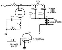
Figure 2-39. - Typical thyratron gas-tube modulator.
The hydrogen thyratron modulator provides improved timing because the synchronized trigger pulse is applied to
the control grid of the thyratron (V2) and instantaneous firing is obtained. In addition, only 2-40
| - |
Matter, Energy,
and Direct Current |
| - |
Alternating Current and Transformers |
| - |
Circuit Protection, Control, and Measurement |
| - |
Electrical Conductors, Wiring Techniques,
and Schematic Reading |
| - |
Generators and Motors |
| - |
Electronic Emission, Tubes, and Power Supplies |
| - |
Solid-State Devices and Power Supplies |
| - |
Amplifiers |
| - |
Wave-Generation and Wave-Shaping Circuits |
| - |
Wave Propagation, Transmission Lines, and
Antennas |
| - |
Microwave Principles |
| - |
Modulation Principles |
| - |
Introduction to Number Systems and Logic Circuits |
| - |
- Introduction to Microelectronics |
| - |
Principles of Synchros, Servos, and Gyros |
| - |
Introduction to Test Equipment |
| - |
Radio-Frequency Communications Principles |
| - |
Radar Principles |
| - |
The Technician's Handbook, Master Glossary |
| - |
Test Methods and Practices |
| - |
Introduction to Digital Computers |
| - |
Magnetic Recording |
| - |
Introduction to Fiber Optics |
| Note: Navy Electricity and Electronics Training
Series (NEETS) content is U.S. Navy property in the public domain. |
|