|
July 1946 Radio-Craft
 [Table of Contents] [Table of Contents]
Wax nostalgic about and learn from the history of early electronics.
See articles from Radio-Craft,
published 1929 - 1953. All copyrights are hereby acknowledged.
|
Fred Shunaman, author of the
two-part "Nomograph Construction" article in Radio-Craft magazine (c1946),
notes that the nomogram is "equal to an infinite number of charts."
Part I covered
the basics of nomograph construction with voltage, current, and resistance.
Part II discusses strategies for best placement and scale types to use for
optimizing the accuracy and usefulness of a nomograph. An inset key is added to
guide the user on how to interpret the results. Figures 1 through 4 and
Nomographs A and B are in Part I.
Part II - Charts with Complicating Factors or Constants
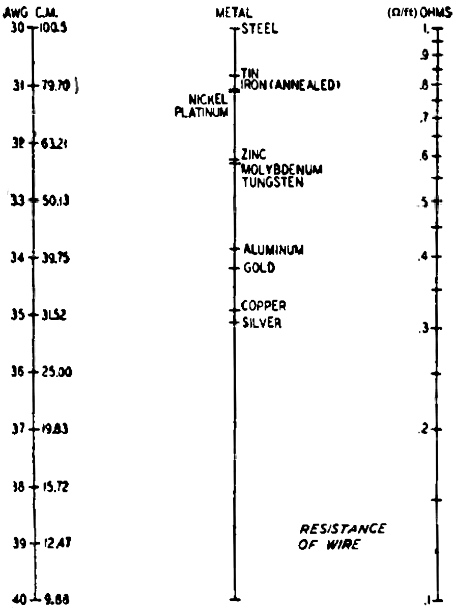
Fig. 5 - Crude chart showing wire resistance.
By Fred Shunaman
The difference between nomographic charts and ordinary graphs is that instead
of having a fixed curve on paper cross-ruled in the quantities which enter a problem,
any such curve can be selected by simply laying a ruler across the two lines which
represent these quantities. This is why a nomogram, is "equal to an infinite number
of charts." Obviously it is more useful than a fixed-curve graph in any problem
in which it can be employed.
The simpler types of nomograms have already been dealt with, and the reader told
how he can construct his own charts to cover any such problems. Somewhat more difficult
constructions are often necessary, or may be found to give a better construction
than the simple methods given in Part I.
In many nomograms, the figures which appear in the finished job are not the actual
quantities being measured. This is to some extent true even in the multiplication
chart, the simplest of nomograms. The two outside scales are evenly divided in logarithmic
lengths, but we ignore them, and merely put down the numbers for which they stand.
We may wish, for example, to construct a nomogram showing the resistance of various
kinds and sizes of wire. The formula is R = k l/C.M.
k being the specific resistivity of the wire (varying for different metals) l, the length in feet, and C.M. the area in circular mils. In this case,
we calculate in circular mils but put down wire sizes in our finished chart. The
specific resistivity and C.M. of all common metals and wire sizes are obtainable
from tables available in many handbooks. It is necessary to construct a chart which
will show the resistance for various areas, lengths and metals.
Our equation can be simplified by letting l length = 1. The chart
will then read resistance per foot, and the equation will be R = k/C.M.
This can be expressed in the form C.M. x R = k. C.M. and R. can then be the outside
scales of a nomogram and k the center one. Laying out one of the outside lines with
the C.M. areas of wire from size 30 to 40 (a 10 to 1 ratio) and the other in resistance
values from 0.1 to 1.0 ohms per foot, the center line is calibrated with the help
of a table of specific resistivity. Beginning with the lowest, silver (9.56) and
copper (10.35) we go on to steel, approximately 100 (varying with the type of
steel). The result appears in Fig. 5.
This chart is hardly satisfactory. Only half the middle scale is used. The range
of wire sizes is very small. We cannot measure anything larger than No. 30. Important
metals with high specific resistivity, such as nichrome and Constantin, do not appear.
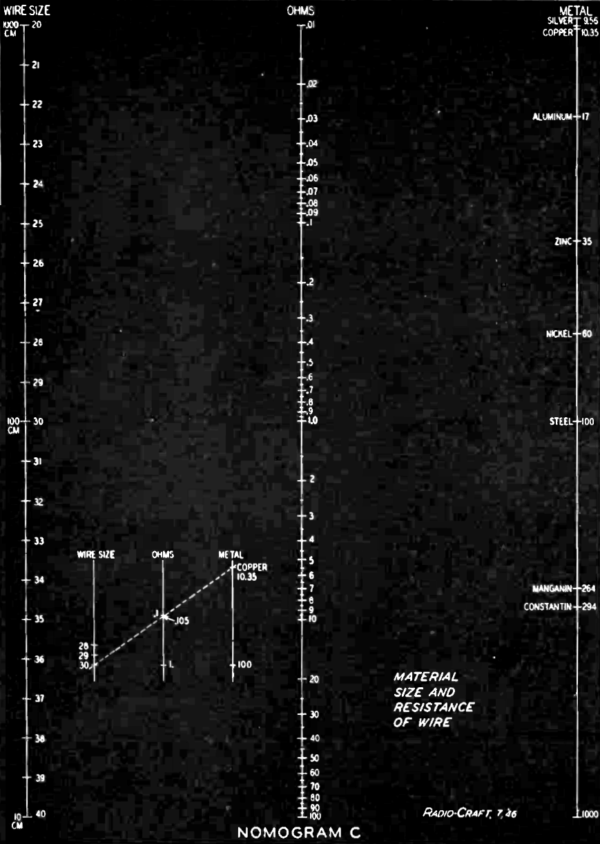
Obviously it would be better to put the k scale outside, where it would cover twice
its present length, and use the center scale for resistance in ohms. This can
be done by changing our equation to R = k x l/C.M. (A reciprocal scale
like 1 /C.M. can be made on a nomogram by simply turning the scale upside down)
Now k and 1 /C.M. can be the outside scales and R the middle one.
Since the resistivity of silver is slightly less than 10 and that of Constantin
near 300, our outside scales should have two cycles. This makes it possible for
the C.M. scale to cover all wire sizes from 20 to 40 (most of the sizes commonly
used in radio). The center scale will again have a range of four cycles.
It is convenient to run down a column of wire sizes, so the C.M. scale is left
as it is and the other two reversed.
Resistivity of silver is very slightly less than 10. Therefore the k scale can
run from 10 to 1,000. Top of the center scale (Nomogram C) marks the resistance
of a wire 1,000 C.M. in diameter and having a specific resistivity of 10.

Material Size and Resistance of Wire Nomograph

Capacity, Frequency, and Inductance Nomograph
This resistance is .01 ohm. The base shows the resistance of a hypothetical wire
with a resistivity of 1,000 and area of 10 circular mils. This is 100 ohms. Graduating
this center scale in four cycles, from .01 to 100 ohms, the C.M. scale from 10 to
1,000, and spotting the k scale with the resistivity of the various metals in which
we are interested, from silver at 9.56 (it is necessary to extend the scale slightly
for this) to Constantin at 296, we have a chart which will cover most of the sizes
and materials used in radio work.
Numbers representing the wire sizes are now inserted on the C.M. scale and the
circular mil figures (which are of no interest) are erased. Thus our nomogram, which
started out with three sets of figures, ends up with only one, the other two scales
being calibrated in wire sizes and names of metals.
If it is desired to extend the range to cover larger sizes of wire, the C.M.
scale may be made into a double one. Readings may then be made from Nos. 1 to 40
(A.W.G. or B&S gage). If the figures on the R scale are read in ohms per hundred
feet instead of ohms per foot, no change need be made in it. The completed graph
is Nomogram C shown on page 700.
Still another type of nomogram is one in which one or more of the factors is
multiplied by a constant, such as A x 4B = C. Since multiplication on a logarithmic
scale is simple addition, we just start the B scale at 4. If the problem were A
x B = 4C, the center scale would start at 4.
One of the best examples of this type of nomogram shows the inductance and capacitance
required to tune to a given frequency. The formula is the well-known
f = 1/ (6.28 √LC) .
The units are farads, henrys and cycles. To get the problem into microhenrys
and microfarads - the practical units of radio - we can multiply numerator and denominator
by 1,000,000, giving
f (cycles) = 1,000,000 /
(6.28 √LμH CμF)
and by dividing the 6.28 into 1,000,000 we can further simplify it to
f (cycles) = 159,000 / √LμH CμF
The frequency in cycles is then equal to 159,000 times
1 / √LC
in microhenrys and in microfarads.
On the nomogram, inductance and capacitance run in opposite direction to the
frequency scale, since the greater the product of the two, the smaller is the number
of cycles per second. The "product" scale will differ from those previously drawn.
Though it is in the center, it will have the same number of cycles as the "factor"
scales. This is because we are using the square roots of the factors. (If Fig. 2,
in the June issue, were to represent the product of the square roots of numbers
from 1 to 10 it would be necessary only to number the three scales identically.)
Then a line drawn through any two numbers on the outside scales would show on the
center one the product of their square roots. (A line through 9 and 4 would cut
the center line at 6, the product of their square roots, 3 and 2.)
For most work where lumped constants are used, it is seldom necessary to calculate
circuits with inductances of less than 10 microhenrys or capacities less than 10
µµf. Using two-cycle paper with these quantities for a base for the two outside
scales, we have a top of 1,000 microhenrys or micromicrofarads. (See Nomogram D,
on opposite page.)
It is a simple matter to calculate calibration points on the center scale by
our equation,
f = 159,000 / √LμH CμF
10 µh and 10 µµf (.00001 µf) are the bases of the two outside scales. 10
µh X .00001 µf = .0001. The square root of this is .01, which divided into 159,000
gives us 15,900,000 cycles, or 15,900 kc. Making the same calculations at the 100
points (100 µh X .0001 (if) and at the top of the scale give us 1,590 kc and 159
kc respectively. From these we can obtain -with the help of 2-cycle papers complete
calibration from 169 to 15,000 kc. Thus the finished chart (Nomogram D) will serve
for practically all i.f., standard broadcasting and international shortwave broadcasting
frequencies.
By clipping the top of our scales at 500 kc and increasing them proportionately
at the bottom, the nomogram could be made to cover all frequencies from the broadcast
band to 50 megacycles. This is done by starting out with three - cycle paper, then
cutting the finished chart down to whatever size is necessary for mounting, publication
or other purposes.
More complex charts may be constructed. A common one has four elements (A X B
X C= D.) The straight edge can cross only two lines to obtain one product, so it
is necessary to work such a chart in two steps. First, A X B = Q, then Q X C = D.
Since it is not necessary to know what the product Q is (because we are interested
only in D) such nomograms have an uncalibrated "Reference line" which is the Q scale
just mentioned. The product of A and B is located on this line with a light pencil
mark, which is used with line C to give the solution on scale D.
Other nomograms (usually beyond the ability of the beginner to construct) combine
multiplication with addition by making one of the factors a composite number containing
one of the factors and the added term. Others represent one or the other of the
quantities by a curved line, and can represent factors which vary other than in
a linear mathematical manner. Some of the simpler of these may be handled in a forthcoming
article.
Posted December 26, 2022
Nomographs / Nomograms Available on RF Cafe:
-
Parallel Series Resistance Calculator -
Transformer Turns Ratio Nomogram -
Symmetrical T and H Attenuator Nomograph -
Amplifier Gain Nomograph -
Decibel
Nomograph -
Voltage and Power Level Nomograph -
Nomograph Construction -
Nomogram Construction for Charts with Complicating Factors or Constants
-
Link Coupling Nomogram -
Multi-Layer Coil Nomograph
-
Delay Line Nomogram -
Voltage, Current, Resistance, and Power Nomograph -
Resistor Selection Nomogram -
Resistance and Capacitance Nomograph -
Capacitance Nomograph -
Earth
Curvature Nomograph -
Coil Winding Nomogram -
RC Time-Constant Nomogram -
Coil Design
Nomograph -
Voltage, Power, and Decibel Nomograph -
Coil Inductance Nomograph -
Antenna Gain Nomograph
-
Resistance and Reactance Nomograph -
Frequency / Reactance Nomograph
|