X-Parameters for Non-Linear Analysis^©

By Kirt Blattenberger, RF Engineer, RFCafe.com webmaster

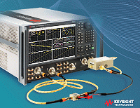
1. Introduction

X-parameters are a frequency-domain behavioral modeling framework for nonlinear RF and microwave components. They were introduced commercially by Agilent Technologies, now Keysight Technologies, as an extension of the earlier Polyharmonic Distortion, or PHD, modeling theory developed by Jan Verspecht, David Root, and collaborators. X-parameters are often described as the nonlinear equivalent of S-parameters, but that phrase must be understood carefully: X-parameters generalize the wave-based, port-oriented language of S-parameters to large-signal, harmonic-rich, nonlinear operating conditions, but they are not a universal, exact, global description of every possible nonlinear behavior. This article only scratches the surface of x-parameters.

For a linear network, S-parameters relate incident traveling waves to reflected or transmitted traveling waves by a linear matrix equation:

b_i = Σ_j S_ija_j

For a nonlinear network driven strongly at one or more frequencies, the output wave at one port and harmonic can depend on the input waves at many ports and harmonics, on the amplitude of the large drive, on bias, on terminations, and on phase relationships. X-parameters address this by describing the nonlinear device around a specified large-signal operating point, or LSOP. The standard single-tone X-parameter formulation contains three principal families of coefficients:

• X^F: the large-signal generated response of the device at each port and harmonic.
• X^S: the small-signal linearized response to incident waves around the large-signal operating point.
• X^T: the conjugate or phase-reversed response term, needed because nonlinear RF behavior generally depends on both a small perturbation and its complex conjugate.

In compact form, for a single large sinusoidal drive at port 1, harmonic 1, the X-parameter expression is commonly written as:

B_p,h = X_p,h^FP^h + Σ_q,k X_p,h;q,k^SP^h-kA_q,k + Σ_q,k X_p,h;q,k^TP^h+kA_q,k^*

where A_q,k is an incident wave at port q and harmonic k, B_p,h is an outgoing wave at port p and harmonic h, P = A_1,1 / |A_1,1| is the phase of the large drive, and the asterisk denotes complex conjugation.

X-parameters are valuable because they allow nonlinear devices such as power amplifiers, mixers, frequency multipliers, driver amplifiers, limiters, and transistors to be represented as measurement-based black-box models. They can be inserted into circuit simulators, cascaded with matching networks, and used in harmonic-balance simulation without revealing the internal transistor-level design. They are especially useful when a device is operated in compression, where ordinary small-signal S-parameters no longer describe gain, phase shift, harmonic generation, load sensitivity, or AM-to-PM conversion accurately.

However, X-parameters are not perfect global nonlinear models. They are normally valid only over the measured or simulated range of bias, frequency, drive level, temperature, port terminations, and modulation conditions. A conventional static X-parameter model assumes a repeatable periodic steady state and a smooth local response around the large-signal operating point. Memory effects, thermal dynamics, trapping, bias-network transients, chaotic behavior, noise, device aging, and unmeasured harmonics may require extended models or other modeling methods.

Important foundational references include Kurokawa’s power-wave formalism for microwave networks, Jan Verspecht and David Root’s Polyharmonic Distortion model, and the book X-Parameters: Characterization, Modeling, and Design of Nonlinear RF and Microwave Components by Root, Verspecht, Horn, and Marcu. See Kurokawa, "Power Waves and the Scattering Matrix," IEEE Transactions on Microwave Theory and Techniques, 1965, Verspecht and Root, "Polyharmonic Distortion Modeling," IEEE Microwave Magazine, 2006, and Root et al., X-Parameters, Cambridge University Press, 2013.

2. Key findings

• X-parameters are a nonlinear, large-signal extension of the wave-based S-parameter concept, but they are not simply "S-parameters at high power."
• The theoretical foundation of X-parameters is Polyharmonic Distortion modeling, developed to describe nonlinear components in the frequency domain using traveling waves at multiple harmonics.
• The principal inventors and developers were not a single person but a group of researchers and engineers, especially Jan Verspecht and David E. Root, with important commercial development at Agilent Technologies, now Keysight Technologies.
• A standard X-parameter model is centered on a large-signal operating point defined by frequency, input power, bias, temperature, and sometimes load condition.
• The model predicts not only the fundamental output but also harmonic generation, nonlinear gain compression, AM-to-PM conversion, port mismatch behavior, and sensitivity to small perturbing signals.
• The X^F terms describe the large-signal response generated by the nonlinear device itself.
• The X^S terms are similar in spirit to S-parameters: they describe how small incident waves affect outgoing waves around the nonlinear operating point.
• The X^T terms have no ordinary small-signal S-parameter equivalent; they describe conjugate mixing caused by nonlinearities and are essential for accurate phase-sensitive nonlinear modeling.
• At sufficiently small signal levels, for a linear time-invariant device, the X-parameter formulation collapses toward ordinary S-parameter behavior.
• X-parameters are most accurate for interpolation within the measured or simulated data set. Extrapolation beyond the characterized range is risky.
• X-parameters are especially important for RF power amplifier design because power amplifiers often operate intentionally in compression for efficiency.
• They can be generated either from nonlinear vector network analyzer measurements or from circuit simulation, commonly harmonic-balance simulation.
• Standard X-parameters describe deterministic large-signal behavior, not random noise by themselves.
• Static single-tone X-parameters may not fully describe memory effects caused by bias networks, thermal phenomena, trapping, or wideband modulated signals. Dynamic or envelope-domain extensions may be required.
• The term "X-parameters" is associated with Keysight/Agilent’s implementation and file ecosystem, whereas the broader theoretical category is nonlinear frequency-domain behavioral modeling or Polyharmonic Distortion modeling.

3. Detailed analysis with sub-headings

3.1 Why S-parameters work so well for linear RF design

To appreciate X-parameters, it is helpful to begin with the reason S-parameters became dominant in microwave engineering. At low frequencies, networks are often described by voltages and currents using impedance, admittance, hybrid, or transmission matrices. At microwave frequencies, directly measuring voltage and current at a device terminal becomes difficult because distributed effects, transmission-line modes, connector launches, standing waves, and calibration planes matter greatly.

S-parameters solve this problem by describing a network in terms of incident and outgoing traveling waves. For a network with real reference impedance Z₀, often 50 Ω, one common power-wave definition is:

a = (V + Z₀I) / (2√Z₀)

b = (V - Z₀I) / (2√Z₀)

where a is the incident wave and b is the outgoing wave. For real Z₀, the net power entering the port is:

P_net = |a|² - |b|²

This power-wave approach is associated with Kurokawa’s classic formulation; see Kurokawa, "Power Waves and the Scattering Matrix," IEEE Transactions on Microwave Theory and Techniques, 1965. A generalized waveguide circuit theory was later formalized by Marks and Williams at NIST; see Marks and Williams, "A General Waveguide Circuit Theory," Journal of Research of NIST, 1992.

For a linear time-invariant network, the outgoing waves are linear combinations of the incident waves:

b₁ = S₁₁a₁ + S₁₂a₂ + ... + S_1Na_N

b₂ = S₂₁a₁ + S₂₂a₂ + ... + S_2Na_N

or in matrix form:

b = Sa

For a two-port:

S-parameters are powerful because they are modular. One can measure a device, store the S-parameter file, insert it into a simulator, cascade it with other networks, design matching networks, and predict system behavior. But this convenience rests on a critical assumption: linearity.

3.2 Why S-parameters fail for nonlinear large-signal operation

A nonlinear RF device does not obey superposition. If an amplifier is driven into compression, doubling the input power does not double the output voltage. The gain changes with drive level, the phase shift may change with amplitude, harmonics are generated, and the apparent input and output impedances may vary with signal level.

For a nonlinear two-port, the output wave may behave conceptually as:

b₂ = f(a₁, a₂, bias, frequency, temperature, load, history, ...)

This is not equivalent to:

b₂ = S₂₁a₁ + S₂₂a₂

A power amplifier operated near saturation is an obvious example. Its small-signal S₂₁ may predict 20 dB gain, but at high input power the amplifier may deliver only 2 dB more output power for a 6 dB increase in input power. At the same time, the output phase may shift with drive amplitude, creating AM-to-PM conversion. Its second and third harmonics may become significant. Its behavior may also change when the load reflection coefficient changes.

For this reason, small-signal S-parameters are insufficient for many modern RF and microwave design problems, especially:

• RF power amplifier design.
• Driver amplifier compression analysis.
• Transistor large-signal characterization.
• Frequency multipliers.
• Mixers and converters.
• Limiters and nonlinear protection circuits.
• RFIC and MMIC behavioral modeling.
• System-level simulation with nonlinear blocks.
• Design using harmonic terminations or load-pull data.

X-parameters were created to preserve the useful wave-based and modular character of S-parameters while extending the framework to nonlinear, harmonic-generating behavior.

3.3 Historical development

3.3.1 Before X-parameters: large-signal measurement and nonlinear simulation

Before X-parameters, nonlinear RF engineers relied on several separate methods:

• Large-signal power sweeps: gain compression, saturated power, P_1dB, efficiency.
• Harmonic measurements using spectrum analyzers.
• Load-pull and source-pull measurements to determine optimum impedances.
• Nonlinear compact transistor models used in harmonic-balance simulators.
• Volterra-series methods for weakly nonlinear systems.
• Behavioral models fitted to measured data.

Each method had value, but none provided a universal equivalent of the S-parameter data block for nonlinear devices. Load-pull data could show optimum impedances but was not a compact multiport behavioral model. Harmonic-balance device models required knowledge of the internal device physics or circuit topology. Spectrum-analyzer data showed output spectra but not calibrated incident and outgoing waves at all ports. Volterra models were useful for mildly nonlinear systems but became cumbersome for strongly nonlinear compressed power amplifiers.

Large-Signal Network Analyzer, or LSNA, technology developed in the 1990s was an important precursor. LSNA and later nonlinear vector network analyzer, or NVNA, systems allowed calibrated measurement of complex traveling waves at the fundamental and harmonics. This made it possible to measure not only output power but also phase-coherent voltage and current waveforms at device ports. Jan Verspecht and collaborators were central figures in this area.

3.3.2 Polyharmonic Distortion modeling

The direct theoretical ancestor of X-parameters is the Polyharmonic Distortion, or PHD, model. The PHD model describes a nonlinear device in terms of frequency-domain traveling waves at a fundamental frequency and its harmonics. The word "polyharmonic" emphasizes that the model includes multiple harmonics, not just the fundamental.

Verspecht and Root described this framework in "Polyharmonic Distortion Modeling," IEEE Microwave Magazine, 2006. The PHD approach recognizes that a nonlinear device driven by a strong periodic signal settles, under suitable conditions, into a periodic steady state. That periodic waveform can be represented by Fourier components at the fundamental and harmonic frequencies. The device can therefore be characterized by relationships among incident and outgoing waves at those harmonic frequencies.

3.3.3 Commercial introduction of X-parameters

Agilent Technologies commercialized the X-parameter concept as a measurement and simulation technology, integrating it with nonlinear vector network analysis and Advanced Design System, ADS. Agilent later separated its electronic measurement business as Keysight Technologies, so modern X-parameter documentation and instrument support are associated with Keysight. Keysight’s RF and microwave nonlinear measurement ecosystem is connected with instruments such as the PNA-X network analyzer family; see Keysight PNA-X network analyzers.

The most authoritative book-length source is Root, Verspecht, Horn, and Marcu, X-Parameters: Characterization, Modeling, and Design of Nonlinear RF and Microwave Components, Cambridge University Press, 2013. This book presents the theory, measurement methods, and applications of X-parameters in detail.

3.3.4 Who invented X-parameters?

It is most accurate to say that X-parameters were not the invention of one isolated individual. The theoretical and measurement foundations came from work on large-signal network analysis and PHD modeling, especially by Jan Verspecht and David E. Root. Commercial implementation and naming as "X-parameters" came from Agilent Technologies, with significant contributions from Root, Verspecht, Jason Horn, Mihai Marcu, and other Agilent/Keysight collaborators.

Thus:

3.4 Basic definitions

Port: A terminal pair or waveguide access point through which RF power enters or leaves a network.

Incident wave, A or a: A traveling wave directed into a device port.

Outgoing wave, B or b: A traveling wave leaving a device port.

Reference impedance, Z₀: The impedance used to define the traveling waves, commonly 50 Ω.

Harmonic index: If the large drive frequency is f₀, harmonic h corresponds to frequency h f₀.

Large-signal operating point, LSOP: The operating condition about which the nonlinear device is characterized. It includes at least frequency, drive amplitude, phase reference, bias, and temperature. Depending on the model, it may also include load condition, source condition, and other state variables.

X^F term: The generated large-signal output wave at a port and harmonic when the device is driven at the LSOP.

X^S term: A linearized coefficient describing how a small incident perturbation wave affects an outgoing wave around the LSOP.

X^T term: A linearized coefficient describing how the complex conjugate of a small incident perturbation affects an outgoing wave. It captures phase-conjugate mixing effects caused by nonlinearity.

P term: A phase-normalizing factor equal to the phase of the large input wave:

P = A_1,1 / |A_1,1| = e^jφ

The factor P is used because if the phase of the large drive is shifted by φ, the h-th harmonic response shifts by hφ.

3.5 The core mathematical idea

Consider a nonlinear RF component driven by a large sinusoidal signal at port 1 and fundamental frequency f₀. Because the device is nonlinear, it may produce outgoing waves at many harmonics:

B_1,1, B_2,1, B_1,2, B_2,2, B_1,3, B_2,3, ...

where the first subscript is the port and the second subscript is the harmonic. For example:

• B_2,1 is the outgoing wave at port 2 at the fundamental frequency.
• B_2,2 is the outgoing wave at port 2 at the second harmonic.
• B_1,3 is the outgoing wave at port 1 at the third harmonic.

The nonlinear scattering relationship can be written abstractly as:

B = F(A, A^*)

The presence of A^* is important. A nonlinear RF system described in complex-envelope form is not generally an analytic function of the complex incident wave alone. It may depend on both the wave and its complex conjugate. This is why X-parameters require the conjugate X^T terms.

A full nonlinear function F could be impossibly complicated. X-parameters simplify the problem by expanding the behavior around a large-signal operating point. For small perturbations around that operating point, the response can be approximated by a first-order expansion in both the perturbation and its conjugate. This is conceptually similar to a Jacobian linearization, except that complex conjugate terms are included.

In general form:

ΔB ≈ J_AΔA + J_A*ΔA^*

The X-parameter coefficients are essentially a physically organized, phase-normalized, harmonic-indexed version of this large-signal response plus the associated Jacobian terms.

3.6 Standard single-tone X-parameter equation

For a single large sinusoidal drive at port 1, harmonic 1, a common X-parameter equation is:

B_p,h = X_p,h^FP^h + Σ_q,k X_p,h;q,k^SP^h-kA_q,k + Σ_q,k X_p,h;q,k^TP^h+kA_q,k^*

Definitions:

The summations are taken over the incident small-signal perturbation waves included in the model. In many practical single-tone models, the large drive wave itself is treated specially as the independent LSOP variable, so the summation terms describe additional small incident waves or reflections around that large drive.

3.7 Physical meaning of the three X-parameter families

3.7.1 X^F: the generated large-signal response

The X^F term tells what the nonlinear device produces at each output port and harmonic under the specified large-signal drive, assuming the reference incident perturbation conditions used during characterization.

For a two-port amplifier driven at port 1, the fundamental output at port 2 is approximately:

B_2,1 ≈ X_2,1^FP

The second-harmonic output at port 2 is:

B_2,2 ≈ X_2,2^FP²

The third-harmonic output at port 2 is:

B_2,3 ≈ X_2,3^FP³

The powers associated with these waves are, for power-normalized waves:

P_out,h = |B_2,h|²

if the port is terminated in the reference impedance and wave normalization is in √W.

3.7.2 X^S: the direct small-signal response around the LSOP

The X^S terms behave most like ordinary S-parameters. They describe how a small incident wave at one port and harmonic affects an outgoing wave at another port and harmonic, while the device is already operating under a large drive.

For example, X_2,1;2,1^S describes how a small incident wave at the output port, at the fundamental frequency, affects the outgoing wave at the output port, also at the fundamental. This is a large-signal output reflection-like quantity, but it is not identical to small-signal S₂₂ measured with the amplifier uncompressed.

3.7.3 X^T: the conjugate response

The X^T terms are one of the most important differences between X-parameters and ordinary S-parameters. They represent the dependence of an outgoing wave on the complex conjugate of an incident perturbation.

In a linear time-invariant network, if a small incident wave is multiplied by e^jθ, the response is also multiplied by e^jθ. There is no dependence on e^-jθ. In a nonlinear system around a pumped operating point, perturbations can mix with the large signal and its harmonics. This produces phase-sensitive effects that require conjugate terms.

A simple conceptual example is a nonlinear relation:

y = c₁x + c₃|x|²x

If x is perturbed around a large value x₀, let:

x = x₀ + δx

Then:

|x|²x = x x^* x

The first-order perturbation contains terms proportional to both δx and δx^*. Therefore a complete local linearization of a nonlinear complex RF relationship requires both direct and conjugate sensitivities.

3.8 Matrix and tensor interpretation

People often refer to an "X-parameter matrix," but strictly speaking X-parameters are more than a single matrix. They are a collection of indexed coefficients that depend on operating conditions.

If we collect all outgoing waves into a vector B and all small incident perturbation waves into a vector A, the model can be written compactly as:

B = X^F + X^SA + X^TA^*

This expression hides the phase-normalizing P factors for readability, but it shows the structure. A still more explicit augmented matrix form is:

[ B ]    [ X^F ]    [ X^S   X^T ] [ A ]
[ B^* ] = [ X^F* ] + [ X^T*   X^S* ] [ A^* ]

This augmented representation makes clear that the conjugate terms double the effective variable set. It also shows why the X-parameter model is related to a Jacobian of the nonlinear scattering function around a large-signal operating point.

For N ports and H harmonics, the number of wave components is approximately:

M = N H

The X^F set contains roughly M complex generated-wave terms. The X^S and X^T sets each contain roughly M × M complex coefficients, although practical models often omit terms that are not relevant or not measured.

3.9 Relationship between X-parameters and S-parameters

X-parameters reduce to S-parameter-like behavior under small-signal, linear conditions. For a linear time-invariant network:

B = SA

There is no harmonic generation, no dependence on drive amplitude, and no conjugate response. Therefore:

• X^S corresponds to the ordinary S-parameter matrix for the relevant fundamental-frequency terms.
• X^T is zero.
• X^F represents the response caused by the selected large incident drive, and in a purely linear device this response is simply proportional to that drive.
• No additional harmonics are generated.

The following table summarizes the comparison:

3.10 Why the phase factor P is necessary

Suppose a nonlinear device is driven by:

A_1,1 = |A_1,1|e^jφ

The fundamental output phase follows the input phase approximately as e^jφ. The second harmonic follows as e^j2φ. The third harmonic follows as e^j3φ. In general, the h-th harmonic response rotates as:

e^jhφ

If this predictable phase dependence were stored directly in the X-parameter coefficients, the coefficients would depend on arbitrary choice of input phase reference. The phase factor:

P = e^jφ

removes this arbitrary dependence. The coefficient X_p,h^F then depends on drive amplitude, frequency, bias, and other real operating variables, not on the arbitrary absolute phase of the large tone.

This is also why the perturbation terms contain powers such as P^h-k and P^h+k. These phase exponents enforce the correct phase covariance between input perturbations and output harmonics.

3.11 How X-parameters are measured

X-parameters can be obtained from either measurement or simulation. In measurement, a nonlinear vector network analyzer is used to measure calibrated complex traveling waves at multiple harmonics. A conventional VNA measures linear S-parameters by applying one small signal at a time. An NVNA or LSNA-style system extends this by measuring large-signal waveforms and harmonic components with phase coherence.

A simplified measurement sequence is:

1. Define the device under test. Specify the number of ports, frequency range, bias conditions, power range, expected harmonics, temperature, and safe operating limits.
2. Calibrate the measurement system. Calibration must establish the measurement reference planes and the magnitude and phase of incident and outgoing waves at the fundamental and harmonics. Calibration is more demanding than ordinary small-signal VNA calibration because harmonic phase information is needed.
3. Apply the large drive. Drive the DUT at the fundamental frequency and selected power level, establishing the LSOP.
4. Measure the generated waves. Measure outgoing waves at each port and harmonic. These data form the basis of the X^F terms.
5. Apply small perturbations. Inject small additional incident waves at selected ports and harmonics while maintaining the large drive. Vary the perturbation phase and possibly amplitude.
6. Solve for the linearized coefficients. The changes in outgoing waves are used to extract the X^S and X^T terms.
7. Sweep operating variables. Repeat for frequency, input power, bias, temperature, and possibly load impedance.
8. Store the model. The resulting data are stored in a format usable by a nonlinear circuit simulator.
9. Validate the model. Compare model predictions with independent measurements such as power sweeps, harmonic powers, load-pull contours, or modulated-signal measurements.

In simulation, the same conceptual process can be performed using harmonic-balance analysis of a nonlinear transistor-level or circuit-level model. The simulator computes the large-signal operating point and then extracts the linearized harmonic response around that point.

3.12 Practical uses of X-parameters

Power amplifier design: X-parameters allow an amplifier or transistor to be characterized under compressed operation and then used in a simulator with external matching networks. This is one of their most important applications.

Harmonic prediction: Since X-parameters include harmonic-indexed waves, they can predict second-harmonic and third-harmonic output levels better than small-signal models.

Load mismatch analysis: The X^S and X^T terms allow prediction of how reflected waves from a nonideal load alter the device’s output.

AM-to-AM and AM-to-PM conversion: As input amplitude changes, X^F changes in magnitude and phase. This captures gain compression and phase distortion.

Cascaded nonlinear system simulation: X-parameter blocks can be inserted into larger circuits and simulated with filters, matching networks, couplers, antennas, and other components.

Vendor model distribution: A manufacturer can distribute a behavioral model of a proprietary MMIC or packaged amplifier without disclosing transistor dimensions, bias architecture, or internal matching topology.

Design-space exploration: Engineers can evaluate how a nonlinear block behaves with different source and load impedances, bias points, or drive levels.

Frequency-conversion devices: Extended X-parameter and PHD-like formulations can be applied to mixers, multipliers, and other periodically driven nonlinear devices, though multi-tone and conversion cases are more complex than the simplest single-tone amplifier case.

3.13 Example: using X-parameters to predict output power with a mismatched load

This example is simplified but illustrates the practical value of the X^S and X^T terms. Suppose a two-port amplifier is characterized at:

• Frequency: 2.0 GHz.
• Bias: fixed at the manufacturer’s recommended operating point.
• Input drive level: a compressed large-signal operating point.
• Reference impedance: 50 Ω.
• Large-signal input phase chosen such that P = 1.

Assume the measured or simulated X-parameter values at the fundamental output are:

With a perfect 50 Ω load, there is no reflected incident wave at the output port, so:

B_2,1 = X_2,1^FP = 0.707 √W

The output power is:

P_out = |B_2,1|² = 0.707² = 0.500 W

In dBm:

P_dBm = 10 log₁₀(0.500 / 0.001) = 26.99 dBm

Now suppose the load is mismatched with reflection coefficient:

Γ_L = 0.20 ∠ 45°

The incident wave returning from the load is:

A_2,1 = Γ_LB_2,1

The X-parameter expression for the output wave is:

B_2,1 = X_2,1^FP + X_2,1;2,1^SA_2,1 + X_2,1;2,1^TP²A_2,1^*

Since P = 1 and A_2,1 = Γ_LB_2,1:

B = C + SΓB + TΓ^*B^*

where:

• B = B_2,1
• C = X_2,1^FP
• S = X_2,1;2,1^S
• T = X_2,1;2,1^T
• Γ = Γ_L

Define:

s = SΓ

t = TΓ^*

Then:

B = C + sB + tB^*

Rearrange:

(1 - s)B - tB^* = C

Solving the two coupled equations for B and B^* gives:

B = [ (1 - s^*)C + tC^* ] / [ |1 - s|² - |t|² ]

Using the numerical values:

SΓ = (0.10 ∠ -20°)(0.20 ∠ 45°) = 0.020 ∠ 25°

TΓ^* = (0.03 ∠ 60°)(0.20 ∠ -45°) = 0.006 ∠ 15°

The resulting output wave is approximately:

B ≈ 0.721 √W

Therefore:

P_out ≈ |0.721|² = 0.520 W

P_dBm ≈ 10 log₁₀(0.520 / 0.001) = 27.16 dBm

The mismatch has increased the predicted output power slightly in this simplified case. With a different load phase, it could decrease output power or change the output phase. This example shows why nonlinear load-dependent modeling requires more than a single compressed gain number. The reflected wave interacts with the nonlinear operating point through both direct and conjugate paths.

3.14 Example design workflow for a novice engineer

Suppose you are designing an RF power amplifier stage using a vendor-supplied X-parameter model. A practical workflow is:

1. Collect model information. Obtain the X-parameter model file, supported frequency range, power range, bias conditions, harmonic order, reference impedance, and simulator compatibility information from the vendor.
2. Verify operating range. Make sure your intended frequency, input drive, supply voltage, temperature, and load VSWR are inside the characterized range. Do not assume the model is reliable outside that range.
3. Insert the X-parameter block into a nonlinear simulator. Use a harmonic-balance simulator that supports the model format.
4. Add bias networks and matching networks. Place realistic input and output matching circuits, DC feeds, decoupling, and package or board parasitics around the X-parameter block as appropriate.
5. Run a matched-load power sweep. Plot output power, gain, phase, power-added efficiency if supported, and harmonic powers versus input power.
6. Identify compression behavior. Determine small-signal gain, P_1dB, saturated output power, and AM-to-PM conversion.
7. Evaluate harmonic content. Check second- and third-harmonic output levels. Modify harmonic terminations if the model and design permit harmonic tuning.
8. Test load mismatch sensitivity. Sweep load reflection coefficient magnitude and phase. Observe output power, phase, harmonic content, and potential instability indicators.
9. Optimize matching networks. Use the nonlinear response, not merely small-signal S-parameters, to optimize the match for desired output power, efficiency, or linearity.
10. Validate with measurements. Build or measure a prototype. Compare measured compression, harmonic levels, and load sensitivity to simulation. If there is disagreement, check whether the real operating conditions differ from the model conditions.

3.15 X-parameters and load-pull

Load-pull is a measurement technique in which the load impedance presented to a device is varied systematically while measuring output power, efficiency, gain, distortion, or other quantities. It is widely used for power amplifier design. X-parameters and load-pull are related but not identical.

Traditional load-pull data are often presented as contours on a Smith chart. They answer questions such as: "What load impedance gives maximum output power?" or "What load gives maximum efficiency?" X-parameters attempt to create a behavioral model that can be used inside a simulator with arbitrary surrounding networks. Load-dependent X-parameter measurements or models can include the effect of changing output termination.

For high-power amplifiers whose behavior changes strongly with load impedance, a simple X-parameter model measured only at a 50 Ω load may be insufficient for large load variations. Load-dependent X-parameters or complementary load-pull data may be necessary.

3.16 X-parameters, harmonic balance, and circuit simulation

Harmonic balance is a frequency-domain nonlinear simulation method widely used in RF design. It assumes that the steady-state waveform can be represented by a finite set of sinusoidal frequency components. Linear parts of the circuit are solved in the frequency domain, while nonlinear device equations are handled through transformations between time and frequency domains.

X-parameters fit naturally into harmonic-balance simulation because they are already frequency-domain, harmonic-indexed behavioral models. Instead of solving internal transistor equations, the simulator uses the X-parameter relationship among incident and outgoing waves.

This gives several advantages:

• The model can be faster than a detailed transistor-level model.
• The model can protect vendor intellectual property.
• The model can be based directly on measurement.
• The model can include package and internal matching behavior automatically if characterized that way.
• The same model can be embedded in larger RF system simulations.

But there are also disadvantages:

• The model is limited to characterized operating conditions.
• It may not reveal internal voltage or current stress.
• It may not predict behavior under unusual bias, temperature, or failure conditions.
• It may not enforce all physical constraints outside the measured data range.

3.17 Are X-parameters a perfect nonlinear equivalent of S-parameters?

The short answer is no. They are an extremely useful nonlinear extension of S-parameter thinking, but they are not a perfect global representation of arbitrary nonlinear device behavior.

Where X-parameters are strong:

• They use the same incident/outgoing wave language familiar to microwave engineers.
• They handle harmonics explicitly.
• They describe compressed large-signal behavior.
• They can model phase-sensitive nonlinear effects through X^T.
• They are measurement-based and therefore can model devices whose internal details are unknown.
• They work well in harmonic-balance design environments.
• They are especially effective for periodic steady-state RF behavior around characterized operating points.

Where X-parameters are limited:

• Locality: Standard X-parameter models are local or regional models around measured large-signal operating points. They are not guaranteed outside that region.
• Finite harmonic truncation: Only a finite number of harmonics are measured or simulated. Real nonlinear devices generate more harmonics than the model includes.
• Interpolation and extrapolation: Interpolation inside a dense measured grid may be accurate; extrapolation outside the grid may be wrong.
• Memory effects: Static X-parameters do not automatically capture long-term thermal, trapping, bias-network, or envelope-memory effects unless the model is extended to include them.
• Wideband modulation: A single-tone X-parameter model may not fully predict adjacent-channel distortion or memory effects under complex modulated signals.
• Noise: Standard deterministic X-parameters do not by themselves describe noise figure, phase noise, or stochastic nonlinear noise behavior.
• Multiple operating states: Some nonlinear circuits can have hysteresis, oscillation, bifurcation, or multiple stable solutions. A simple X-parameter table may not capture all possible states.
• Strong perturbations: The X^S and X^T terms are small-signal linearizations around an LSOP. If the perturbing incident waves are large, higher-order terms may be needed.
• Stability and causality constraints: Ensuring that a behavioral model remains physically valid in every external circuit can be difficult.

A useful way to state the matter is:

X-parameters can accurately represent the measured nonlinear scattering behavior of a device within a specified operating domain and under the assumptions of the model, but they are not an all-condition physical law for the device.

3.18 Why the model depends on the large-signal operating point

In a linear network, S-parameters ideally do not depend on signal amplitude. In a nonlinear device, the operating point changes with drive level. Consider gain compression. The large-signal gain can be written as:

G(P_in) = P_out(P_in) / P_in

At small signal:

G(P_in) ≈ G₀

Near compression:

G(P_in) < G₀

Therefore the output wave coefficient must depend on |A_1,1|. Similarly, AM-to-PM conversion means output phase also depends on drive amplitude:

∠B_2,1 = φ_linear + φ_AM-PM(|A_1,1|)

Thus X-parameters are functions of operating variables:

X = X(f₀, |A_1,1|, V_bias, I_bias, T, Γ_S, Γ_L, ...)

Different X-parameter data sets may be required for different bias points, temperatures, frequency bands, or load-pull conditions.

3.19 X-parameters and AM-to-AM / AM-to-PM conversion

AM-to-AM conversion describes how output amplitude changes with input amplitude. AM-to-PM conversion describes how output phase changes with input amplitude. Both are central in RF power amplifier design.

Using the fundamental large-signal output:

B_2,1 = X_2,1^F(|A_1,1|)P

The large-signal power gain is:

G_P = |B_2,1|² / |A_1,1|²

Substituting:

G_P = |X_2,1^F(|A_1,1|)|² / |A_1,1|²

The output phase relative to the input is:

φ_out-in = ∠X_2,1^F(|A_1,1|)

As |A_1,1| is swept, changes in the magnitude of X^F reveal AM-to-AM behavior, while changes in its phase reveal AM-to-PM behavior.

3.20 X-parameters and harmonic generation

A nonlinear device driven at f₀ may produce output at:

f₀, 2f₀, 3f₀, 4f₀, ...

The harmonic output powers can be predicted from:

P_out,h = |B_2,h|²

If no additional perturbing incident waves are present:

B_2,h ≈ X_2,h^FP^h

Therefore:

P_out,h ≈ |X_2,h^F|²

This makes X-parameters useful for predicting harmonic levels, filter requirements, and spectral purity. However, the prediction is only as good as the harmonic order included in the model and the accuracy of the terminations used during characterization and simulation.

3.21 Multi-tone and dynamic X-parameters

The simplest X-parameter model is single-tone and static: one large fundamental drive, periodic steady state, and harmonic components. Real communication systems often use modulated signals with wide bandwidth. In such cases, the envelope changes with time, and the device may exhibit memory effects.

Memory effects can arise from:

• Thermal time constants.
• Bias-network charging and discharging.
• Trapping effects in semiconductor devices.
• Frequency-dependent matching and package effects.
• Baseband impedance interactions.

For modulated signals, a device’s instantaneous output may not be determined solely by the instantaneous input amplitude. It may also depend on previous values:

y(t) = F[x(t), x(t - τ₁), x(t - τ₂), temperature(t), bias(t), ...]

Static X-parameters may still be useful, especially for narrowband or quasi-static behavior, but dynamic X-parameter extensions or other behavioral models may be needed for accurate prediction of adjacent-channel power ratio, error vector magnitude, digital predistortion behavior, and memory-induced distortion.

The literature distinguishes between the core PHD/X-parameter concept and extensions for mixers, converters, modulated signals, and dynamic behavior. The exact terminology may vary among vendors and authors, so engineers should inspect model documentation carefully rather than assuming every "X-parameter" file supports every nonlinear effect.

3.22 Comparison with other nonlinear modeling approaches

3.23 Practical cautions when using X-parameter models

• Check the reference impedance. Most RF models use 50 Ω, but do not assume this blindly.
• Check harmonic order. A model including only three harmonics cannot predict fifth-harmonic behavior.
• Check input power range. Do not use a model characterized up to +20 dBm to predict +30 dBm drive unless the vendor explicitly supports that extrapolation.
• Check bias conditions. X-parameters measured at one drain voltage or collector voltage may not be valid at another.
• Check temperature. Power devices can be strongly temperature dependent.
• Check load conditions. A 50 Ω characterized model may not be reliable for severe mismatch or harmonic load tuning.
• Check stability. Behavioral models may not expose all internal oscillation mechanisms.
• Check modulation validity. Single-tone X-parameters may not predict wideband modulated performance accurately.
• Validate against measurements. Always compare simulation to measured power, gain, phase, harmonics, and distortion where possible.

4. Open questions / debates in the field

4.1 Standardization and interoperability

S-parameters have the widely used Touchstone format. X-parameters have been more closely tied to vendor-specific ecosystems and nonlinear simulator support. A continuing practical question is how open, portable, and standardized nonlinear behavioral model formats should be. Engineers benefit when models can move easily between measurement systems and simulators, but vendors also have incentives to maintain differentiated toolchains.

4.2 How best to include memory effects

Static X-parameters are highly effective for periodic steady-state behavior, but many modern RF systems use wideband modulated signals. Memory effects can dominate adjacent-channel distortion and digital predistortion performance. There remains active engineering interest in how best to combine wave-based nonlinear models with dynamic envelope, thermal, trapping, and baseband-memory effects.

4.3 Validity under severe mismatch

Power amplifiers may encounter high-VSWR loads in real systems. A model characterized near 50 Ω may not remain valid under severe mismatch. Load-dependent X-parameter models help, but the measurement burden grows quickly as frequency, power, bias, harmonic terminations, and load reflection coefficient are swept.

4.4 Measurement complexity and uncertainty

Accurate nonlinear vector measurements require demanding calibration, harmonic phase references, power calibration, and uncertainty management. Compared with ordinary S-parameter measurements, X-parameter extraction is more complex. A continuing question is how to make these measurements more repeatable, traceable, and accessible.

4.5 Physical constraints in black-box models

A black-box behavioral model may interpolate measured data well but still behave nonphysically outside the measured region. Ensuring passivity where appropriate, causality, stability, energy conservation, and physically plausible extrapolation is harder for nonlinear models than for linear S-parameters.

4.6 Noise and stochastic behavior

Standard X-parameters describe deterministic nonlinear scattering. Noise in nonlinear devices, especially under large-signal drive, is a more difficult problem. Engineers may need separate noise models or extended formulations for oscillator phase noise, mixer noise, amplifier noise under compression, and noise conversion.

4.7 Relationship to machine-learning models

Modern behavioral modeling increasingly uses machine learning. Neural-network and data-driven models can fit complex nonlinear behavior, but they may lack the physical interpretability and port-wave structure of X-parameters. A current debate is whether future models should be primarily physics-structured, like X-parameters, purely data-driven, or hybrid.

5. Sources cited inline with links where possible

• K. Kurokawa, "Power Waves and the Scattering Matrix," IEEE Transactions on Microwave Theory and Techniques, 1965. Foundational paper on power waves and scattering matrices.
• R. B. Marks and D. F. Williams, "A General Waveguide Circuit Theory," Journal of Research of the National Institute of Standards and Technology, 1992. Important reference for generalized waveguide and network measurement theory.
• J. Verspecht and D. E. Root, "Polyharmonic Distortion Modeling," IEEE Microwave Magazine, 2006. Core theoretical ancestor of X-parameters.
• D. E. Root, J. Verspecht, J. Horn, and M. Marcu, X-Parameters: Characterization, Modeling, and Design of Nonlinear RF and Microwave Components, Cambridge University Press, 2013. Authoritative book-length treatment of X-parameter theory, measurement, and application.
• Keysight Technologies, PNA-X Network Analyzers. Industry source for nonlinear vector network analysis platforms associated with X-parameter measurement workflows.
• Keysight PathWave Advanced Design System, ADS. Industry simulator ecosystem in which X-parameter nonlinear behavioral models have been widely used.
• National Institute of Standards and Technology, Microwave and Millimeter-Wave Metrology. Official source for microwave measurement science, calibration, and metrology context relevant to VNA/NVNA measurements.

Closing perspective

X-parameters are best understood as a practical bridge between measurement and nonlinear RF simulation. They retain the familiar port-wave viewpoint of S-parameters while adding the large-signal, harmonic, and conjugate-response information needed for nonlinear devices. Their greatest value appears when ordinary S-parameters are no longer meaningful: compressed amplifiers, harmonic-generating devices, nonlinear MMICs, and load-sensitive RF power stages. They are not perfect, and they should not be used casually outside their characterized domain, but within that domain they are one of the most important behavioral modeling tools developed for modern nonlinear microwave engineering.

This content was generated primarily with the assistance of ChatGPT (OpenAI), and/or Gemini (Google), and/or Arya (GabAI), and/or Grok (x.AI), and/or DeepSeek artificial intelligence (AI) engines. Review was performed to help detect and correct any inaccuracies; however, you are encouraged to verify the information yourself if it will be used for critical applications. In all cases, multiple solicitations to the AI engine(s) was(were) used to assimilate final content. Images and external hyperlinks have also been added occasionally - especially on extensive treatises. Courts have ruled that AI-generated content is not subject to copyright restrictions, but since I modify them, everything here is protected by RF Cafe copyright. Many of the images are likewise generated and modified. Your use of this data implies an agreement to hold totally harmless Kirt Blattenberger, RF Cafe, and any and all of its assigns. Thank you. Here is Gab AI in an iFrame.

AI Technical Trustability Update

While working on an update to my RF Cafe Espresso Engineering Workbook project to add a couple calculators about FM sidebands (available soon). The good news is that AI provided excellent VBA code to generate a set of Bessel function plots. The bad news is when I asked for a table showing at which modulation indices sidebands 0 (carrier) through 5 vanish, none of the agents got it right. Some were really bad. The AI agents typically explain their reason and method correctly, then go on to produces bad results. Even after pointing out errors, subsequent results are still wrong. I do a lot of AI work and see this often, even with subscribing to professional versions. I ultimately generated the table myself. There is going to be a lot of inaccurate information out there based on unverified AI queries, so beware.

Electronics & High Tech Companies | Electronics & Tech Publications | Electronics & Tech Pioneers | Electronics & Tech Principles | Tech Standards Groups & Industry Associations | Societal Influences on Technology